Create a complete ggplot for a waveband descriptor.

Construct a ggplot object with an annotated plot of a waveband object.

Usage

# S3 method for class 'waveband'
autoplot(
  object,
  ...,
  w.length = NULL,
  range = NULL,
  fill = 0,
  span = NULL,
  wls.target = "HM",
  unit.in = getOption("photobiology.radiation.unit", default = "energy"),
  unit.out = unit.in,
  annotations = NULL,
  by.group = FALSE,
  geom = "line",
  wb.trim = TRUE,
  norm = NA,
  text.size = 2.5,
  ylim = c(NA, NA),
  object.label = deparse(substitute(object)),
  na.rm = TRUE
)

Arguments

object: a waveband object.
...: arguments passed along by name to autoplot.response_spct().
w.length: numeric vector of wavelengths (nm).
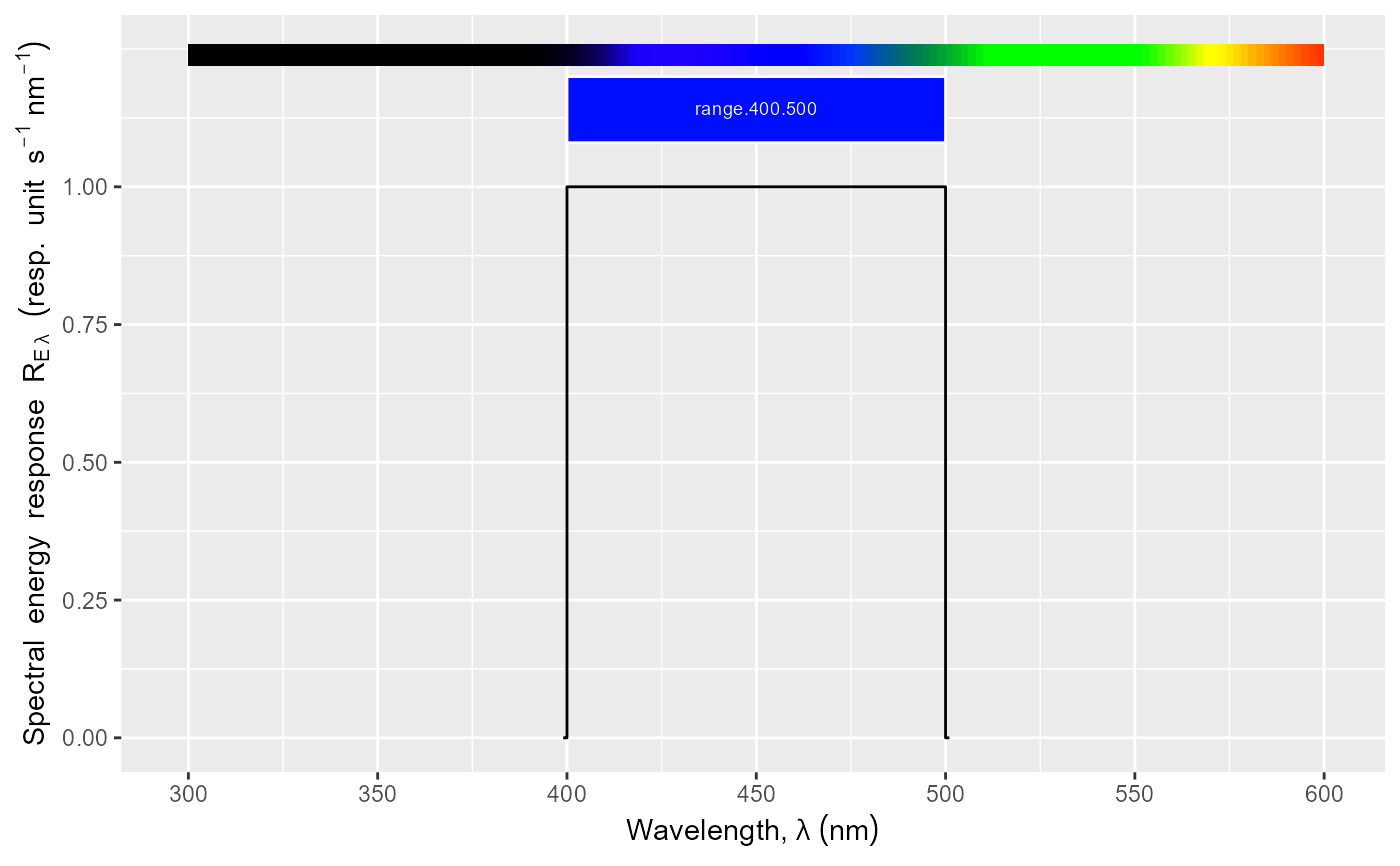
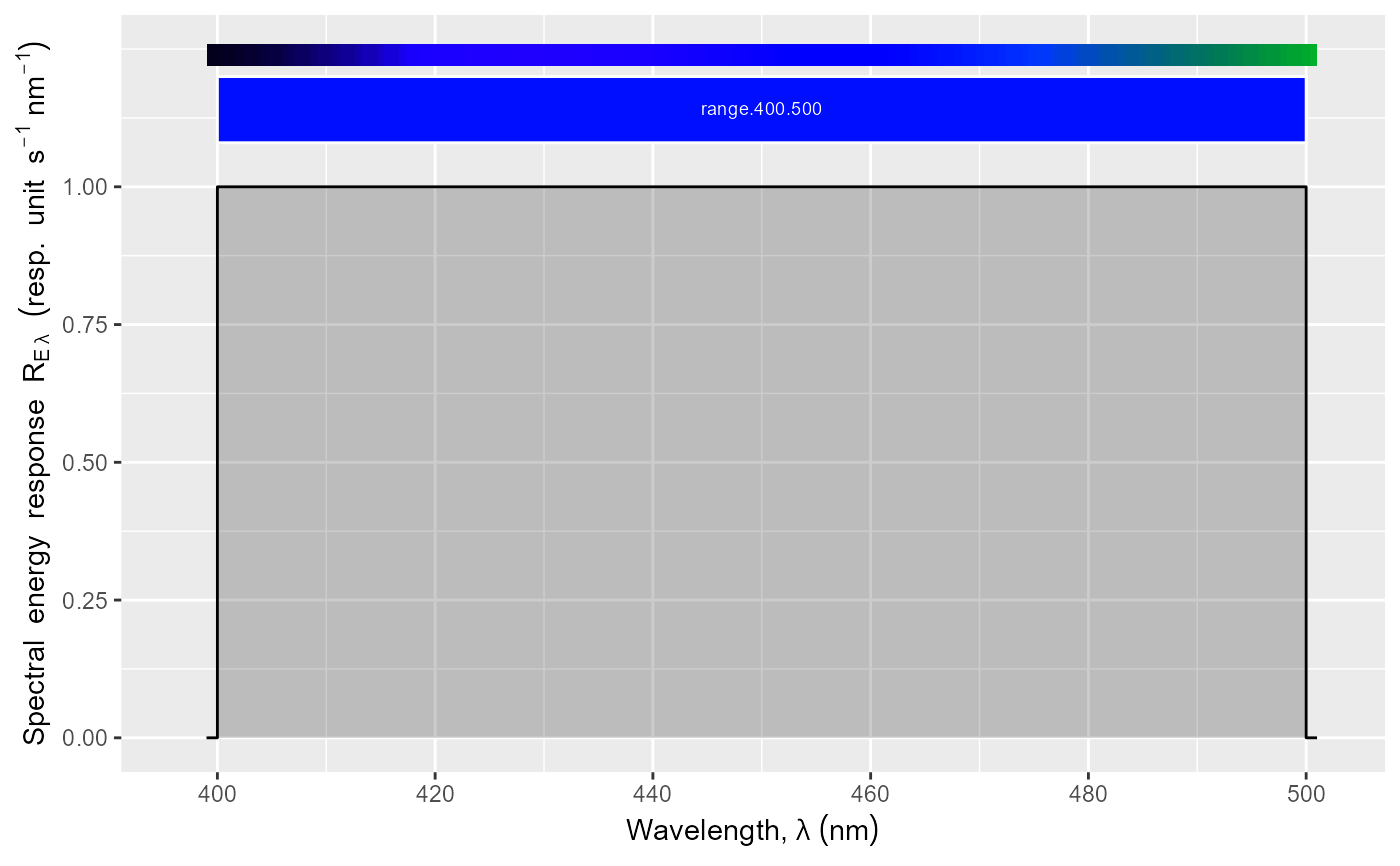
range: an R object on which range() returns a vector of length 2, with min annd max wavelengths (nm).
fill: value to use as response for wavelengths outside the waveband range.
span: a peak is defined as an element in a sequence which is greater than all other elements within a window of width span centered at that element.
wls.target: numeric vector indicating the spectral quantity values for which wavelengths are to be searched and interpolated if need. The character strings "half.maximum" and "half.range" are also accepted as arguments. A list with numeric and/or character values is also accepted.
unit.in, unit.out: the type of unit we assume as reference: "energy" or "photon" based for the waveband definition and the implicit matching response plotted.
annotations: a character vector. For details please see section Plot Annotations.
by.group: logical flag If TRUE repeated identical annotation layers are added for each group within a plot panel as needed for animation. If FALSE, the default, single layers are added per panel.
geom: character The name of a ggplot geometry, currently only "area", "spct" and "line".
wb.trim: logical. Passed to trim_wl. Relevant only when the waveband extends partly outside range.
norm: numeric or character Normalization wavelength (nm) or character string "max" or other criterion for normalization.
text.size: numeric size of text in the plot decorations.
ylim: numeric y axis limits,
object.label: character The name of the object being plotted.
na.rm: logical.

Value

a ggplot object.

Details

A response_spct object is created based on the waveband object and the argument passed to parameter w.length. By default wavelengths spanning the waveband definition expanded by 1 nm at each end are used. A waveband object can describe either a simple wavelength range or a (biological) spectral weighting function (BSWF). An effectiveness is a response expressed per unit of excitation, and in most cases normalised.

Effectiveness spectra can be plotted expressing the spectral effectiveness either per mol of photons (\(1 mol^{-1} nm\)) or per joule of energy (\(1 J^{-1} nm\)), selected through formal argument unit.out. The value of unit.in has no direct effect on the result for BSWFs, as BSWFs are defined based on a certain base of expression, which is enforced. Indirectly it affects plots as unit.out defaults to unit.in. In contrast, for wavebands which only define a wavelength range, changing the assumed reference irradiance units, changes the responsivity according to Plank's law, i.e., the four possible combinations of pairs of values for unit.in and unit.out produce four different plots. _Only in rare cases unit.in and unit.out is useful as normally the dependency on base of expresion is encoded in the waveband definition as a BSWF._

While w.length` provides the wavelengths of the generated response spectrum, `range` sets the wavelength range of the \(x\)-axis of the plot.

Unused named arguments are forwarded to autoplot.response_spct(), allowing control of additional plot properties.

Plot Annotations

The recognized annotation names are: "summaries", "peaks", "peak.labels", "valleys", "valley.labels", "wls", "wls.labels", "colour.guide", "color.guide", "boxes", "segments", "labels". In addition, "+" is interpreted as a request to add to the already present default annotations, "-" as request to remove annotations and "=" or missing"+" and "-" as a request to reset annotations to those requested. If used, "+", "-" or "=" must be the first member of a character vector, and followed by one or more of the names given above. To simultaneously add and remove annotations one can pass a list containing character vectors each assembled as described. The vectors are applied in the order they appear in the list. To disable all annotations pass "" or c("=", "") as argument. Adding a variation of an annotation already present, replaces the existing one automatically: e.g., adding "peak.labels" replaces"peaks" if present.

The annotation layers are added to the plot using statistics defined in 'ggspectra': stat_peaks, stat_valleys, stat_label_peaks, stat_label_valleys, stat_find_wls, stat_spikes, stat_wb_total, stat_wb_mean, stat_wb_irrad, stat_wb_sirrad, stat_wb_contribution, stat_wb_relative, and stat_wl_strip. However, only some of their parameters can be passed arguments through autoplot methods. In some cases the defaults used by autoplot methods are not the defaults of the statistics.

Examples


autoplot(waveband(c(400, 500)))

autoplot(waveband(c(400, 500)), w.length = c(300,600))

autoplot(waveband(c(400, 500)), range = c(300,600))

autoplot(waveband(c(400, 500)), geom = "spct")