Animated plots of spectral data
‘ggspectra’ 0.4.0
Pedro J. Aphalo
2026-03-18
Source:vignettes/articles/animated-plots.Rmd
animated-plots.RmdIntroduction
This article is only available as part of the on-line documentation of R package ‘ggspectra’. It is not installed in the local computer as part of the package.
Package ggspectra extends ggplot2 with
stats, geoms, scales and annotations suitable for light- or
radiation-related spectra. It also defines ggplot() and
autoplot() methods specialized for the classes defined in
package photobiology for storing different types of
spectral data. The autoplot() methods are described
separately in vignette User Guide: 2 Autoplot Methods and the
ggplot() methods, statistics, and scales in User Guide:
1 Grammar of Graphics.
The new elements can be freely combined with methods and functions
defined in packages ‘ggplot2’, scales,
ggrepel, gganimate and other extensions to
‘ggplot2’.
This article, focuses on plots of time-series of spectra created with R package ‘ggspectra’ and animated with package ‘gganimate’. Time series of spectra stored in one of the classes from R package ‘photobiology’ can be acquired or imported easily when using Ocean Optics spectrometers, with R package ‘ooacquire’. Such data can also be obtained with radiation transfer models or other brands of spectrometers and in many cases imported with R package ’photobiologyInOut. Similarly, kinetics of chemical reactions involving light absorbing reactants and/or products as well as any other temporal change in colour and or intensity can be characterised through spectral data. In addition to time, as exemplified below using time-series, other series of measurements in response to changes in other continuous explanatory variables are well suited to animations.
One limitation of the current version of ‘gganimate’ is that it
does not support scales names that are R expressions as
returned by R functions parse() and
expression(). Functions str2lang() and
bquote() have to be used instead. These functions are used
within ‘ggspectra’ (>= 0.3.16) improving compatibility .
‘gganimate’ imposes a couple of restrictions: a) statistics must
generate output for each group in groupings created by mapping
aesthetics to factors, as image frames in animations behave like groups,
b) expressions used as labels when including substitution of values from
data must be defined using bquote() so that the subtitution
takes place at the correct stage in the building of the animations.
Deviations from these requirements made ‘ggspectra’ < 3.16.0
incompatible with ‘gganimate’. These two requirements are now
fulfilled.
A difficulty remains in that within ‘ggspectra’ and
‘photobiology’ the default argument for unit.out is
determined through an R option. When not set, "energy" is
used. This option does not seem to be in all cases visible when an
animation is assembled leading to inconsistencies that break the
animation code when the R option is set to "photon" instead
of "energy". Currently, the solution is to pass
unit.out = "photon" explicitly in the function calls when
creating animations.
Compatibility with ‘gganimate’ is rather fragile, and may break when ‘ggplot2’, ‘gganimate’ or R itself are updated. Thus, long-term compatibility between ‘ggspectra’ and ‘gganimate’ cannot be assured.
Set up
## Loading required package: SunCalcMeeus## Documentation at https://docs.r4photobiology.info/
library(photobiologySun)
library(photobiologyWavebands)
library(ggspectra)
energy_as_default()

library(lubridate)
##
## Attaching package: 'lubridate'## The following objects are masked from 'package:base':
##
## date, intersect, setdiff, union
# if suggested packages are available
gganimate_installed <- requireNamespace("gganimate", quietly = TRUE)
eval_chunks <- gganimate_installed
if (eval_chunks) {
  library(gganimate)
  message("'gganimate' version ", format(packageVersion('gganimate')), " loaded and attached.")
} else {
  message("Please, install package 'gganimate'.")
}
## 'gganimate' version 1.0.11 loaded and attached.
eval_repel <- requireNamespace("ggrepel", quietly = TRUE)
if (eval_repel) {
  library(ggrepel)
  message("'ggrepel' version ", format(packageVersion('ggrepel')), " loaded and attached.")
} else {
  message("Please, install package 'ggrepel'.")
}
## 'ggrepel' version 0.9.7 loaded and attached.We change the default theme.
Using the grammar of graphics
A time series of five spectra
We change the labels in the factor so that the time of measurement can be shown.
my_sun.spct <- sun_evening.spct
time <- when_measured(my_sun.spct, as.df = TRUE)
my_sun.spct$spct.idx <- factor(my_sun.spct$spct.idx,
                               levels = time[["spct.idx"]],
                               labels = as.character(round_date(time[["when.measured"]], unit = "minute")))
summary(my_sun.spct)
## Summary of source_spct [7,965 x 3] object: my_sun.spct
## containing 5 spectra in long form
## Wavelength range 290-1000 nm, step 0.34-0.47 nm
## Label: cosine.hour.9
## time.01 measured on 2023-06-12 18:38:00.379657 UTC
## time.02 measured on 2023-06-12 18:39:00.797266 UTC
## time.03 measured on 2023-06-12 18:40:00.714554 UTC
## time.04 measured on 2023-06-12 18:41:00.768459 UTC
## time.05 measured on 2023-06-12 18:42:00.769065 UTC
## Measured at 60.227 N, 24.018 E; Viikki, Helsinki, FI
## Variables:
## w.length: Wavelength [nm]
## s.e.irrad: Spectral energy irradiance [W m-2 nm-1]
## --
## w.length s.e.irrad spct.idx
## Min. : 290.0 Min. :0.00000 2023-06-12 18:38:00:1593
## 1st Qu.: 474.4 1st Qu.:0.02315 2023-06-12 18:39:00:1593
## Median : 654.8 Median :0.03892 2023-06-12 18:40:00:1593
## Mean : 651.6 Mean :0.03659 2023-06-12 18:41:00:1593
## 3rd Qu.: 830.3 3rd Qu.:0.04888 2023-06-12 18:42:00:1593
## Max. :1000.0 Max. :0.07503We create a base plot to play with:
ggplot(data = my_sun.spct) +
  aes(linetype = spct.idx) +
  geom_line() +
  scale_x_wl_continuous() +
  scale_y_s.e.irrad_continuous()
We can animate a plot in different ways. Here, using long transitions between spectra. During the transitions interpolated data values are used to create an artificial smooth transition.
ggplot(data = my_sun.spct) +
  geom_line() +
  scale_x_wl_continuous() +
  scale_y_s.e.irrad_continuous() +
  transition_states(spct.idx,
                    transition_length = 2,
                    state_length = 1)
The default base of expression for irradiance and spectral irradiance is
"energy", while "photon" (= quantum) is also
supported. Below we edited the plot code immediately above adding
unit.out = "photon" to ggplot() and replacing
y scale scale_y_s.e.irrad_continuous() with
scale_y_s.q.irrad_continuous().
ggplot(data = my_sun.spct, unit.out = "photon") +
  geom_line() +
  scale_x_wl_continuous() +
  scale_y_s.q.irrad_continuous() +
  transition_states(spct.idx,
                    transition_length = 2,
                    state_length = 1)
Next, we add an indication of which spectrum is being displayed. Here we define the title and subtitle of the plot to be dynamic, showing information about the currently displayed frame of the animation.
ggplot(data = my_sun.spct) +
  geom_line() +
  scale_x_wl_continuous() +
  scale_y_s.e.irrad_continuous() +
  transition_states(spct.idx,
                    transition_length = 2,
                    state_length = 1) +
  ggtitle('Now showing {closest_state} UTC',
          subtitle = 'Frame {frame} of {nframes}')
Some statistics have compute functions that work by ggplot panel
instead of by ggplot group to avoid redundant output in regular plots.
To be used in animations, statistics should generate output for each
group, as groups are the basis of the frames in the animation. Starting
from ‘ggspectra’ 3.16.0 statistics that normally produce a single output
per panel have a formal parameter by.group that when passed
TRUE changes their behaviour to repeatedly produce the same
output for each group. A typical example are “annotation-like” output,
like labels for wavebands with stat_wb_label(). These
statistics use the data mostly as reference for positioning and extent,
but not directly. For example, labels for wavebands located
automatically just above the top of the tallest spectrum in a normal
figure panel and “trimmed” to the wavelengths in data. In an animation,
they must be added, instead of once per plot to each individual image
frame, that internally are ggplot groups, rather than panels.
Thus, it is possible to add various annotations. Here energy irradiances for red and far-red light together with labels for the wavebands.
ggplot(data = sun_evening.mspct) +
geom_line() +
stat_wb_label(aes(colour = after_stat(wb.color)),
w.band = list(Red("Sellaro"), Far_red("Sellaro")),
ypos.fixed = 0.082,
by.group = TRUE) + # needed for animation
stat_wb_e_irrad(aes(colour = after_stat(wb.color)),
w.band = list(Red("Sellaro"), Far_red("Sellaro")),
ypos.fixed = 0.078) +
stat_wb_hbar(aes(colour = after_stat(wb.color)),
w.band = list(Red("Sellaro"), Far_red("Sellaro"))) +
scale_x_wl_continuous() +
scale_y_s.e.irrad_continuous() +
scale_colour_identity() +
transition_states(spct.idx,
transition_length = 2,
state_length = 1,
) +
ggtitle('Now showing {closest_state} UTC',
subtitle = 'Frame {frame} of {nframes}')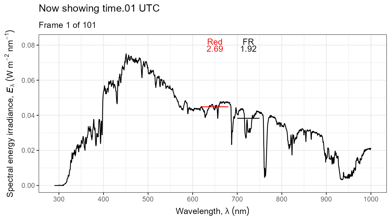 The code above edited to use photons as base of expression by changing
as above, but also adjusting the position of annotations and their
multiplier. While the scale and annotations are expresses in \mu\mathrm{mol}\,\mathrm{m}^{-2}\,\mathrm{s}^{-1}\,\mathrm{nm}^{-1}
the data are stored as \mathrm{mol}\,\mathrm{m}^{-2}\,\mathrm{s}^{-1}\,\mathrm{nm}^{-1}.
The code above edited to use photons as base of expression by changing
as above, but also adjusting the position of annotations and their
multiplier. While the scale and annotations are expresses in \mu\mathrm{mol}\,\mathrm{m}^{-2}\,\mathrm{s}^{-1}\,\mathrm{nm}^{-1}
the data are stored as \mathrm{mol}\,\mathrm{m}^{-2}\,\mathrm{s}^{-1}\,\mathrm{nm}^{-1}.
ggplot(data = sun_evening.mspct, unit.out = "photon") +
  geom_line() +
  stat_wb_label(aes(colour = after_stat(wb.color)),
                w.band = list(Red("Sellaro"), Far_red("Sellaro")),
                ypos.fixed = 0.37e-6, by.group = TRUE) +
  stat_wb_q_irrad(aes(colour = after_stat(wb.color)),
                  w.band = list(Red("Sellaro"), Far_red("Sellaro")),
                  label.mult = 1e6,
                  ypos.fixed = 0.35e-6) +
  stat_wb_hbar(aes(colour = after_stat(wb.color)),
                  w.band = list(Red("Sellaro"), Far_red("Sellaro"))) +
  scale_x_wl_continuous() +
  scale_y_s.q.irrad_continuous() +
  scale_colour_identity() +
  transition_states(spct.idx,
                    transition_length = 2,
                    state_length = 1,
                    ) +
  ggtitle('Now showing {closest_state} UTC',
          subtitle = 'Frame {frame} of {nframes}')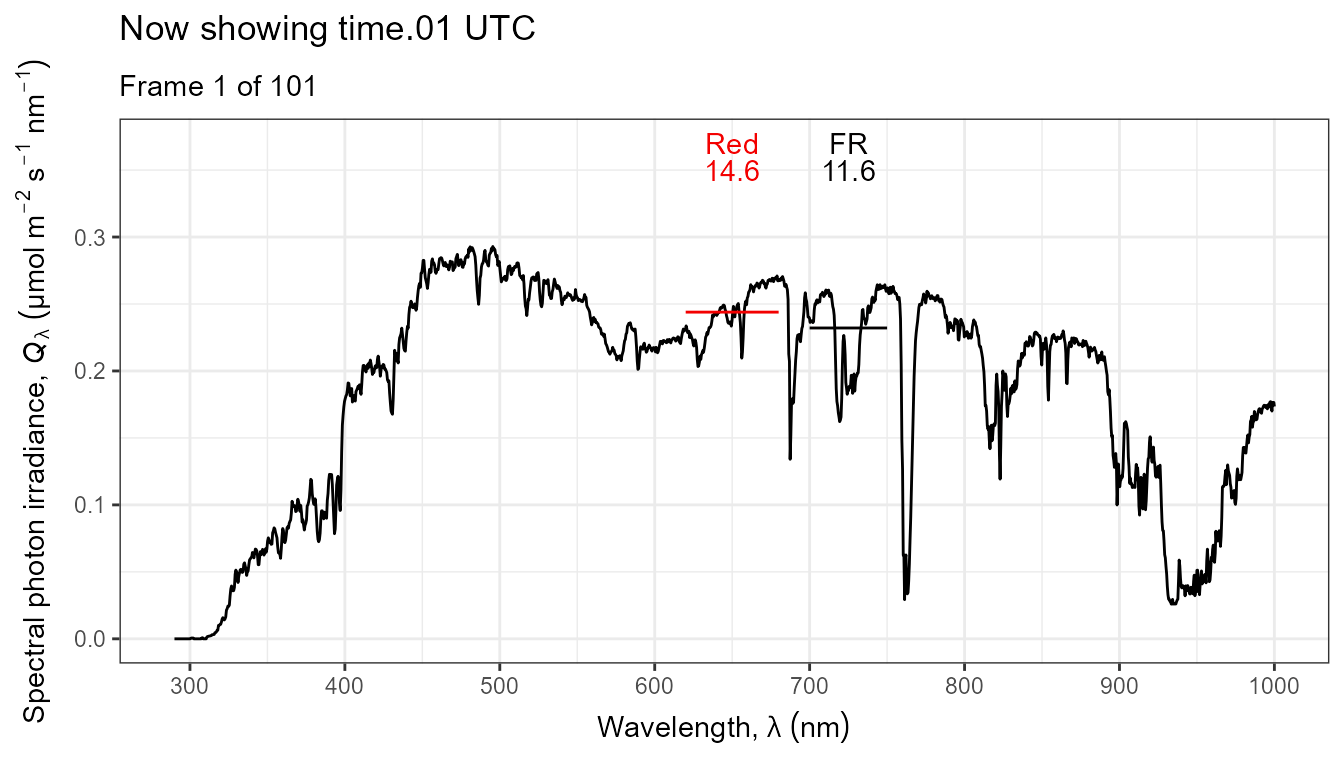
A time series of 15 spectra
With these examples animate() crashed R 4.5.0 with
‘ggplot2’ 3.5.2 and ‘gganimate’ 1.0.9. I do not know where the trouble
originated, however setting the factor describing the times differently
in the spectral data, seems to have made the examples work once again.
There is still one border line example that fails.
Object sun_hourly_august.spct contains multiple spectra
in long form. Variable UTC indicate the date and time for
each spectrum, and factor spct.idx identifies the spectra
using a name. The data included in package ‘photobiologySun’ cover most
of the daytime of two successive days. We select data for one day.
# select data for 21 August
my_sun.spct <-
  subset(sun_hourly_august.spct,
         day(UTC) == 21 & spct.idx != "spct.30")
# number of spectra
getMultipleWl(my_sun.spct)
## [1] 15
# levels of the factor identifying the individual spectra
levels(my_sun.spct[[getIdFactor(my_sun.spct)]])
## [1] "spct.01" "spct.02" "spct.03" "spct.04" "spct.05" "spct.06" "spct.07"
## [8] "spct.08" "spct.09" "spct.10" "spct.11" "spct.12" "spct.13" "spct.14"
## [15] "spct.15"
# summary of spectra
summary(my_sun.spct, expand = "collection")
## Summary of source_mspct [15 x 1] object: anonymous
## # A tibble: 15 × 8
## spct.idx class dim w.length.min w.length.max colnames multiple.wl time.unit
## <chr> <chr> <chr> <dbl> <dbl> <list> <dbl> <Duratio>
## 1 spct.01 sour… [511… 290 800 <chr> 1 1s
## 2 spct.02 sour… [511… 290 800 <chr> 1 1s
## 3 spct.03 sour… [511… 290 800 <chr> 1 1s
## 4 spct.04 sour… [511… 290 800 <chr> 1 1s
## 5 spct.05 sour… [511… 290 800 <chr> 1 1s
## 6 spct.06 sour… [511… 290 800 <chr> 1 1s
## 7 spct.07 sour… [511… 290 800 <chr> 1 1s
## 8 spct.08 sour… [511… 290 800 <chr> 1 1s
## 9 spct.09 sour… [511… 290 800 <chr> 1 1s
## 10 spct.10 sour… [511… 290 800 <chr> 1 1s
## 11 spct.11 sour… [511… 290 800 <chr> 1 1s
## 12 spct.12 sour… [511… 290 800 <chr> 1 1s
## 13 spct.13 sour… [511… 290 800 <chr> 1 1s
## 14 spct.14 sour… [511… 290 800 <chr> 1 1s
## 15 spct.15 sour… [511… 290 800 <chr> 1 1sWe replace the indexing factor with one using local time of day for levels instead of arbitrary names. This makes it easier to display the times in the animations.
# replace the values used for indexing to times of day
my_sun.spct[[getIdFactor(my_sun.spct)]] <-
  factor(format.POSIXct(my_sun.spct[["UTC"]],
                 format = "%H:%M",
                 tz = "Europe/Helsinki"))
# rename the factor used for indexing
setIdFactor(my_sun.spct, "tod")
getIdFactor(my_sun.spct)
## [1] "tod"
summary(my_sun.spct[[getIdFactor(my_sun.spct)]])## 06:30 07:30 08:30 09:30 10:30 11:30 12:30 13:30 14:30 15:30 16:30 17:30 18:30
## 511 511 511 511 511 511 511 511 511 511 511 511 511
## 19:30 20:30
## 511 511
# head
my_sun.spct
## Object: source_spct [7,665 x 4]
## containing 15 spectra in long form
## Wavelength range 290-800 nm, step 1 nm
## Label: Radiation transfer model (LibRadtran) simulation of solar spectrum
## by Anders K. Lindfors
## spct.01 measured on 2014-08-21 03:30:00 UTC
## spct.02 measured on 2014-08-21 04:30:00 UTC
## spct.03 measured on 2014-08-21 05:30:00 UTC
## spct.04 measured on 2014-08-21 06:30:00 UTC
## spct.05 measured on 2014-08-21 07:30:00 UTC
## spct.06 measured on 2014-08-21 08:30:00 UTC
## spct.07 measured on 2014-08-21 09:30:00 UTC
## spct.08 measured on 2014-08-21 10:30:00 UTC
## spct.09 measured on 2014-08-21 11:30:00 UTC
## spct.10 measured on 2014-08-21 12:30:00 UTC
## spct.11 measured on 2014-08-21 13:30:00 UTC
## spct.12 measured on 2014-08-21 14:30:00 UTC
## spct.13 measured on 2014-08-21 15:30:00 UTC
## spct.14 measured on 2014-08-21 16:30:00 UTC
## spct.15 measured on 2014-08-21 17:30:00 UTC
## Measured at 60.20388 N, 24.96082 E; Kumpula, Helsinki, Finland
## Variables:
## w.length: Wavelength [nm]
## s.e.irrad: Spectral energy irradiance [W m-2 nm-1]
## --
## # A tibble: 7,665 × 4
## w.length s.e.irrad UTC tod
## <dbl> <dbl> <dttm> <fct>
## 1 290 0 2014-08-21 03:30:00 06:30
## 2 291 2.85e-11 2014-08-21 03:30:00 06:30
## 3 292 6.49e-10 2014-08-21 03:30:00 06:30
## 4 293 2.84e- 9 2014-08-21 03:30:00 06:30
## 5 294 9.05e- 9 2014-08-21 03:30:00 06:30
## 6 295 2.94e- 8 2014-08-21 03:30:00 06:30
## 7 296 8.70e- 8 2014-08-21 03:30:00 06:30
## 8 297 1.91e- 7 2014-08-21 03:30:00 06:30
## 9 298 4.52e- 7 2014-08-21 03:30:00 06:30
## 10 299 9.78e- 7 2014-08-21 03:30:00 06:30
## # ℹ 7,655 more rows
# summary of spectra
summary(my_sun.spct, expand = "collection")
## Summary of source_mspct [15 x 1] object: anonymous
## # A tibble: 15 × 8
## spct.idx class dim w.length.min w.length.max colnames multiple.wl time.unit
## <chr> <chr> <chr> <dbl> <dbl> <list> <dbl> <Duratio>
## 1 06:30 sour… [511… 290 800 <chr> 1 1s
## 2 07:30 sour… [511… 290 800 <chr> 1 1s
## 3 08:30 sour… [511… 290 800 <chr> 1 1s
## 4 09:30 sour… [511… 290 800 <chr> 1 1s
## 5 10:30 sour… [511… 290 800 <chr> 1 1s
## 6 11:30 sour… [511… 290 800 <chr> 1 1s
## 7 12:30 sour… [511… 290 800 <chr> 1 1s
## 8 13:30 sour… [511… 290 800 <chr> 1 1s
## 9 14:30 sour… [511… 290 800 <chr> 1 1s
## 10 15:30 sour… [511… 290 800 <chr> 1 1s
## 11 16:30 sour… [511… 290 800 <chr> 1 1s
## 12 17:30 sour… [511… 290 800 <chr> 1 1s
## 13 18:30 sour… [511… 290 800 <chr> 1 1s
## 14 19:30 sour… [511… 290 800 <chr> 1 1s
## 15 20:30 sour… [511… 290 800 <chr> 1 1sAll 15 spectra in a single static plot, without using ‘gganimate’. It is not easy to get a sense of how the spectrum varies through the day.
ggplot(data = my_sun.spct) +
  aes(group = tod) +
  geom_line(alpha = 1/3, na.rm = TRUE) +
  scale_x_wl_continuous() +
  scale_y_s.e.irrad_continuous()
The same data as above, but displayed as an animated plot. This plot communicates better the temporal dynamics of spectral irradiance.
getIdFactor(my_sun.spct)## [1] "tod"
anim <- ggplot(data = my_sun.spct) +
  geom_line(na.rm = TRUE) +
  scale_x_wl_continuous() +
  scale_y_s.e.irrad_continuous() +
  transition_states(tod,
                    transition_length = 2,
                    state_length = 1) +
  ggtitle('Now showing {closest_state} local time (EEST)',
          subtitle = 'Frame {frame} of {nframes}')
animate(anim, duration = 20, fps = 10)
To more easily see the differences in the shape of the spectra we can
scale them to an equal total irradiance, 100\,\mathrm{W\,m^{-2}}, i.e., equal area
under each of the curves. To visually emphasize this, we use
geom_spct() instead of geom_line() used in the
examples above.
anim <- ggplot(data = fscale(my_sun.spct, f = e_irrad, target = 100),
               unit.out = "energy") +
  geom_spct(na.rm = TRUE) +
  scale_x_wl_continuous() +
  scale_y_s.e.irrad_continuous(name = s.e.irrad_label(scaled = TRUE)) +
  transition_states(tod,
                    transition_length = 2,
                    state_length = 1) +
  ggtitle('Now showing {closest_state} UTC',
          subtitle = 'Frame {frame} of {nframes}')
animate(anim, duration = 20, fps = 10)
A similar plot as above can be created expressing the spectral irradiance in photon-based units instead of in energy-based units. We scale the spectra to 1\,000\,\mathrm{\mu mol\,m^{-2}\,s{-1}}.
anim <- ggplot(data = fscale(my_sun.spct, f = q_irrad, target = 1e-3),
               unit.out = "photon") +
  geom_spct(na.rm = TRUE) +
  scale_x_wl_continuous() +
  scale_y_s.q.irrad_continuous(name = s.q.irrad_label(scaled = TRUE)) +
  transition_states(tod,
                    transition_length = 2,
                    state_length = 1) +
  ggtitle('Now showing {closest_state} UTC',
          subtitle = 'Frame {frame} of {nframes}')
animate(anim, duration = 20, fps = 10)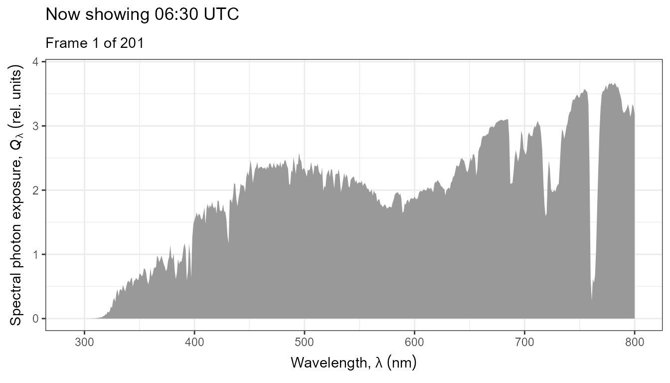
autoplot() support
It is possible to animate ggplots created with
autoplot() methods. However, because in animations “plot
decorations” need to be added by group instead of by panel,
by.group = TRUE has to be added to the call, which is
otherwise as for a static plot. (Internally by.group = TRUE
is passed to the statistics from ‘ggspectra’ that support it, as
described above.).
All label definitions created by functions and methods from
‘ggspectra’ (>= 0.3.16) are static or defined using
bquote() as required by ‘gganimate’.
Currently there is a further limitation: changing the default for
unit.out into "photon" using the R option
results in an error unless it is also passed as argument in the call to
autoplot().
autoplot(my_sun.spct, by.group = TRUE) +
  transition_states(tod,
                    transition_length = 2,
                    state_length = 1)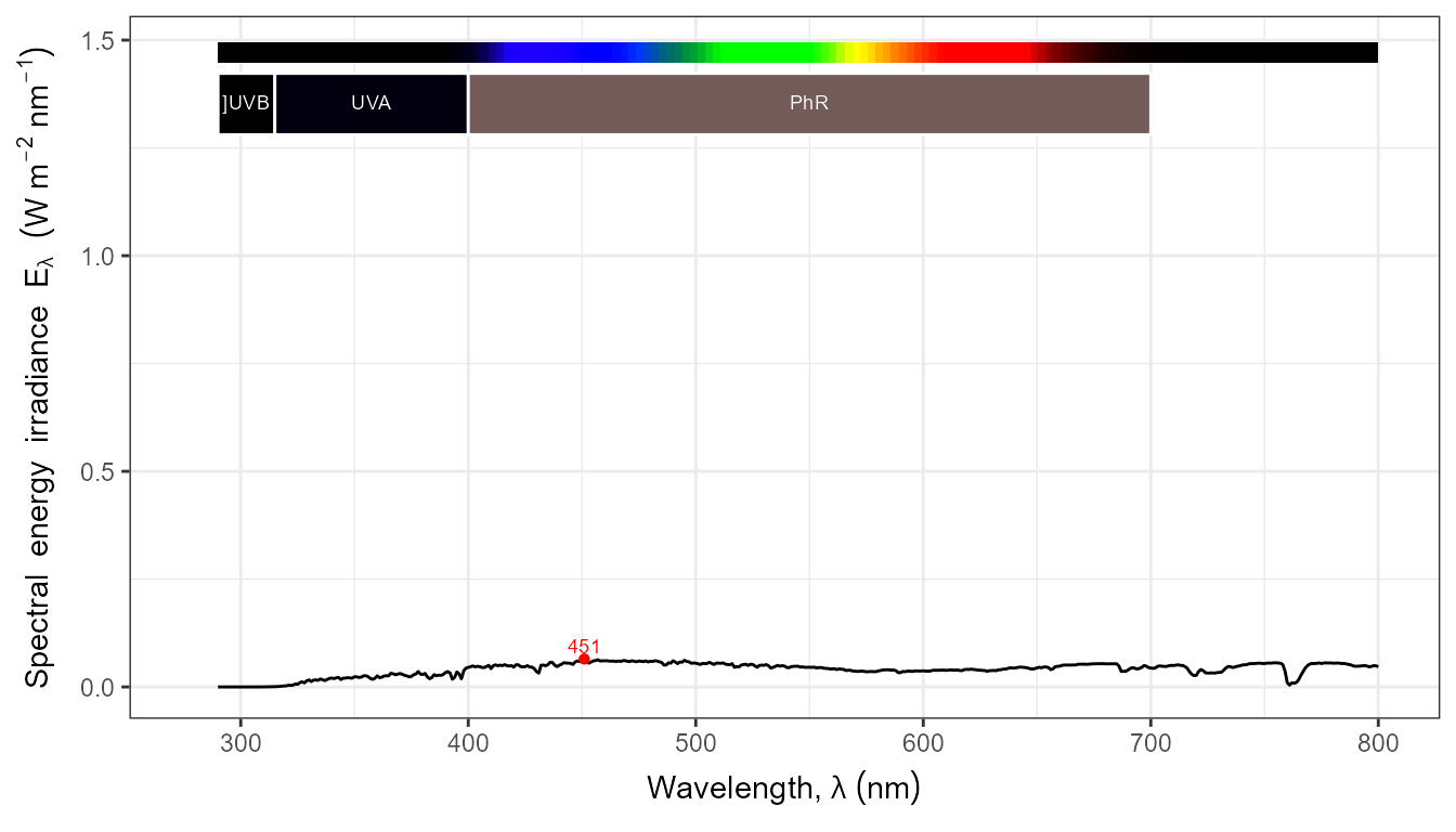
autoplot(my_sun.spct,
         by.group = TRUE,
         geom = "spct",
         span = 51,
         annotations = c("+", "peak.labels")) +
  transition_states(tod,
                    transition_length = 2,
                    state_length = 1)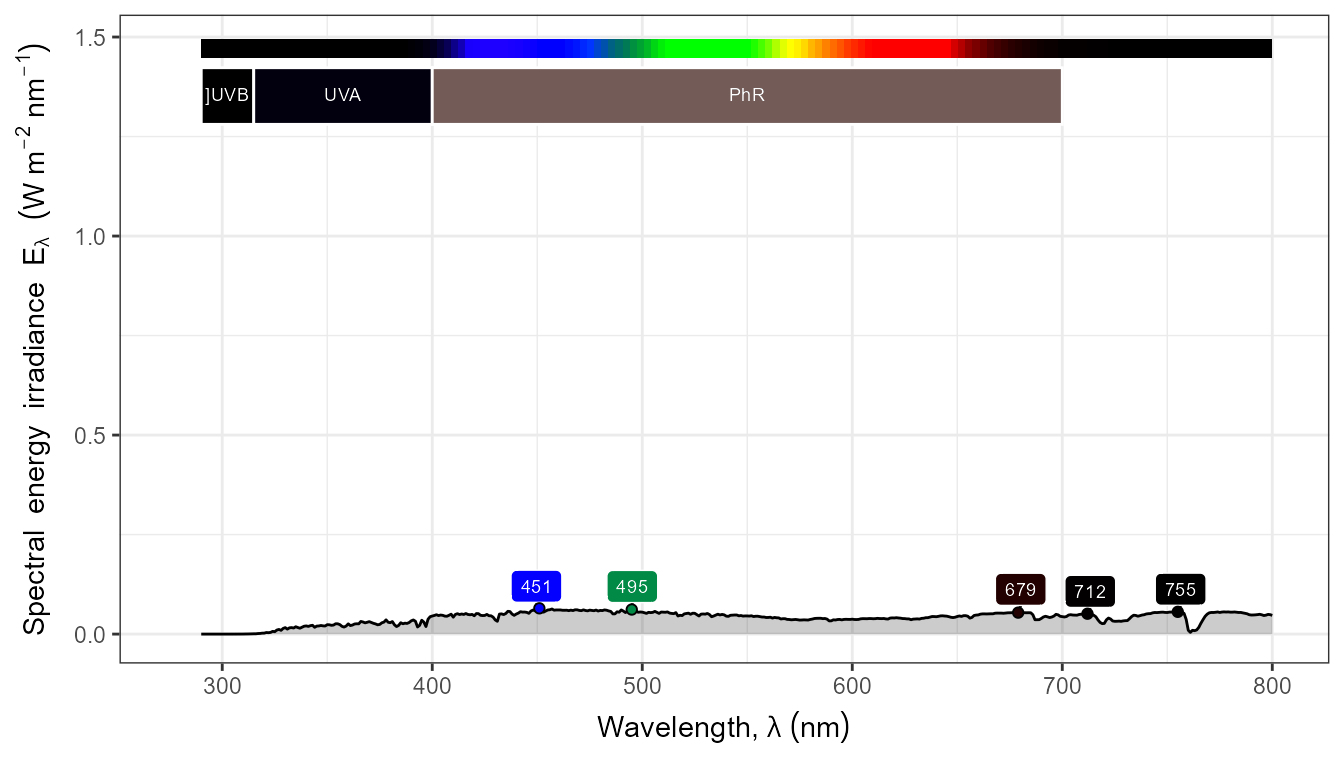
The conversion to photon based units works as expected when set in the call.
autoplot(my_sun.spct, by.group = TRUE, label.qty = "sirrad",
         unit.out = "photon") +
  transition_states(tod,
                    transition_length = 2,
                    state_length = 1)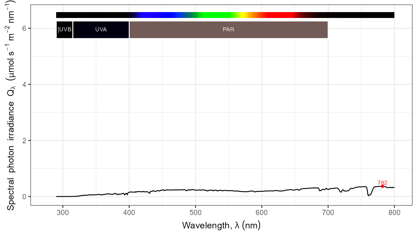
photon_as_default()
autoplot(my_sun.spct, by.group = TRUE) +
  transition_states(tod,
                    transition_length = 2,
                    state_length = 1)