Algorithms
ooacquire
0.4.3.9000
Pedro J. Aphalo
2024-01-13
Source:vignettes/userguide-algorithms.Rmd
userguide-algorithms.RmdIntroduction
In this vignette we will walk through the different steps used in the conversion of raw counts into physical quantities. Different protocols can be used, and not all those implemented are exemplified. The facilities in the package also allow users to implement their own measurement and correction protocols. It must be, however, always kept in mind that protocols and calibrations go hand in hand: For each different measuring protocol or new raw conversion algorithm new calibration multipliers will be required. In the case of new measurement protocols new calibration data and validation measurements will be needed. However, for new raw data conversion protocols recalculation of new calibration multipliers from existing raw-counts and calibration-lamp data may be enough. In this last case existing validation measurements against other instruments can be reused if available.
Preliminaries
We start by loading the R packages we will use.
## Loading required package: photobiology## News at https://www.r4photobiology.info/## Loading required package: lubridate##
## Attaching package: 'lubridate'## The following objects are masked from 'package:base':
##
## date, intersect, setdiff, unionSpectral irradiance from a continuous source
Continuous here means that the length of the integration is determined by the integration time setting in the spectrometer rather than the duration of a light burst. There are many ways in which spectral irradiance data can be acquired with an array spectrometer. The most basic approach is to simply 1) measure a light source and subtract the signal from a few pixels in the array that are not exposed to light (electrical dark). This ignores that the dark signal varies to some extent among individual pixels and also ignores stray light. The most common approach is to 2) acquire paired measurements of a light source and with the input optics blocked or the light source switched off. This ignores stray light. In some cases it is best to 3) measure the light source directly, through a filter and completely blocked/switched-off. If a filter suitable for the source is used and a correction algorithm applied it is possible to discount both the dark signal and stray light. Stray light can be usually subtracted only from a certain region of the spectrum. Finally each of these approaches can be combined with 4) the use of multiple integration times to enhance the dynamic range by splicing different spectra for low and high spectral irradiance regions. In all cases it is possible to 5) acquire multiple “scans” or spectra for each measurement using exactly the same settings and average them pixel by pixel to reduce the noise. In many cases this averaging can be done on board the spectrometer or by the software driver on the host computer.
Table 1 lists the measuring protocols supported. Different approaches in general require separate calibrations of the spectrometer. Some approaches are only applicable to specific types of light sources. It is important to understand that acquisition of each of light, dark and filter measurements is done similarly in the different protocols, so if one has used the “lfd” protocol to acquire the spectra the analysis as “ld” can be done by discarding the measured filter spectrum/spectra.
| Protocol | Light | Dark | Filter | HDR |
|---|---|---|---|---|
| “l” | yes | no | no | yes/no |
| “ld”, “dl” | yes | yes | no | yes/no |
| “lfd”, “dfl” | yes | yes | yes | yes/no |
By using these protocols we obtain raw counts data from the detector array. These need to be converted into spectral irradiance (energy or photon based). Not all detectors behave similarly. For example, for some types of arrays the dark noise increases only for very long integration times while for others more quickly. To be on the safe side even if not strictly necessary, the default acquisition protocols when multiple integration times are used, these multiple times are applied to light, dark and filter measurements.
In addition to these, additional corrections for the shape of the slit function and stray light are possible and implemented in some correction methods. These of course require characterization and calibration of individual spectrometers in more detail than usually done by manufacturers or most users. The corrections implemented are those described by in Yliantilla et al. (2005) and later modified approaches applicable to different models of spectrometers (Ylianttila, unpublished). Package ‘ooacquire’ thus provides a lot of flexibility but the results achieved will depend on the goodness of the calibration, its traceability and the characteristics of the spectrometer and the light source.
A good array spectrometer has a signal to noise ratio of about 1000, and in the best possible case we can improve this by one order of magnitude to 10000 using some of the approaches implemented. This difference is enough to allow measurement of UV-B radiation in sunlight when the sun is several degrees above the horizon, which are otherwise impossible.
A few things to remember:
Pixel resolution is usually higher, sometimes a lot higher, than the true optical resolution of the monochromator grid.
The wavelength step between pixels varies along the array, and by how much depends on the optical configuration.
Array detectors do not respond linearly to the number of photons, so a linearisation correction is always needed.
The digitised data for each pixel is a “count”, i.e., an integer number. The maximum count (related to the number of bits) varies, but it is usually not more that 65000.
In general it is best not to apply boxcar smoothing or re-expression to different wavelengths at an early stage or at all.
Dark noise of the sensor increases with temperature, so some spectrometers have cooled arrays. Spectrometers with no cooling should be shaded from direct sunlight. For accurate measurements spectrometers should be allowed to warm up or cool-down until their temperature is stable.
Temperature of the spectrometer also affects the wavelength calibration, but how much depends on the design of each spectrometer model.
Sometimes we know a priori which wavelengths are not present in a light source and we can take advantage of this to estimate stray light and or for sanity checks. Say if your reading for UV-C in sunlight at ground level is different from zero, this tells that the measurement is bad. (Not that UV-C is being transmitted through the atmosphere.)
Know the limitations of the spectrometer and the protocols you use.
Ylianttila et al.’s (2005) method
I recommend reading the original paper for the details of algorithm
and under which conditions it can be used. It roughly corresponds to the
method named ylianttila in the package, using only
light and dark measurements together with bracketing
of the integration time using a factor of 10. This method was originally
developed for mesurements of sunbeds. This method requires special
characterization of the spectrometer characteristics and a calibration
that is good enough to achieve the additional accuracy. The calibration
is normally done using the same protocol as for measurements and at a
similar temperature. For each type of spectrometer and configuration the
validity of the method needs to be demonstrated by comparison to a
double monochromator scanning spectrometer.
Ylianttila’s (unpublished) method for sunlight
Method ylianttila uses the original stray
light correction algorithm for straylight correction developed by Lasse
Ylianttila for the Maya 2000 Pro based on Ylianttila et al. (2005). The
Maya 2000 Pro suffers from stray light, most notably for sources
emmiting IR with wavelengths > 1000 nm. (Early units seem to have
worse performance in this respect than more recent ones, even for the
same configuration.)
UV-B radiation in sunlight is especially difficult to measure, in general impossible to measure reliably with array spectrometers without a custom sofisticated protocol and correction algorithm. This new method adds a third measurement through a polycarbonate filter (PC). It is crucial to use PC as filter as many other “better” UV blocking filters do not have sufficiently high transmittance in the IR and partly block the stray light. As the PC filter does absorb some visible and IR radiation, about 10-15% for normal incidence, this needs to be compensated as well as any change in incident irradiance between the light and filter measurements. To achieve this the two measurements are compared at wavelengths in the UV-A1 region and the filter measurement rescaled. This works in sunlight or with other continuous spectra but not with discontinuous spectra with low or no radiation in the target region used for rescaling. (When rescaling is not possible a warning is issued and the filter measurement not used.)
The correction for stray light has very little if any effect when measuring UV-A1 or visible radiation. In the case of the Maya 2000 Pro it is also very rarely necessary if the light source emits little or no radiation at wavelengths > 1000 nm. So, when measuring narrow band visible or UV radiation from LEDs, the filter correction is both unnecessary and impossible to apply. With the Maya 2000 Pro there is one situation where correction for stray light would be needed but not possible with this method: measuring a LED emitting at wavelengths > 950 nm.
Other methods
I have implemented a variation on Ylianttila’s method to correct for
stray light named full that differs in the way the ratio
used for rescaling the filter measurement is computed (the
computation is essentially the same as for original but
removing outliers and limiting the range of values for the ratio). This
method should be used only for sunlight or shade light at the Earth
surface. This method uses the same characterization and calibration as
Ylianttila’s method. For situations were the light measurement
has been done under irradiance differeing by more than 10% from that
during the filter measurement, method original
will perform better.
I have implemented a variation on Ylianttila’s method to correct for
stray light named sun that differs in that it sets to zero
spectral irradiance wavelengths shorter than 290 nm. This method should
be used only for sunlight or shadelight at the Earth surface. This
method uses the same characterization and calibration as Ylianttila’s
method.
Method simple uses a simple ad-hoc method to correct for
stray light based on a constant value for the PC filter transmittance.
It is based on light, filter and dark
measurements but no computed rescaling of the filter
measurement is done except multiplication by a contant. It can be
combined with bracketing of integration time even when using a
calibration provided by Ocean Optics or acquired with Ocean Optics’
software.
Method none does not apply any correction for stray
light, is based on a light and dark measurement. It
can be combined with bracketing of integration time even when using a
calibration provided by Ocean Optics or acquired with Ocean Optics’
software. It still applies slit function correction if available, but if
it is not, and is not combined with bracketing of integration time, it
is similar (identical?) to spectral irradiance measured with Ocean
Optics software.
What methods are available
What method can be applied depends on how the spectrometer has been
characterized and calibrated. The deatils of each of the methods need to
be adjusted to each instrument, and the calibration done using the same
corrections or a superset of the corrections used for actual
measurements. For a calibration already expressed as multipliers only
method none is applicable. If the raw counts for the
calibration measurements are available for light,
filter and dark conditions, calibrations for any of
the methods can be constructed. The methods as described include a “tail
correction” for the slit function, based on the characterization of the
slit function at different wavelengths using a laser. This corrections
is most important for sources with narrow peaks such as discharge lamps,
and can be skipped if these data are unavailable.
Examples
We will step through the different stages of the algorithms used, plotting the spectra at each step along the way. We use raw counts data, included in the package, from the measurement of sunlight at ground level with an Ocean Optics Maya 2000 Pro array spectrometer. Before the computations walk-through we will describe how the data and metadata are stored. We will also show the use of a high level function that automatically go through all steps needed to convert raw spectrometer counts into irradiance when a correction method and an instrument calibration are supplied.
We will use photon/quantum units throughout for plotting of spectra and display of computed summaries, while printing remains unaffected. We override the default use of energy units by changing the R option with a convenience function.
The raw counts data and computed spectral irradiance
Spectral data used in this example were acquired using function
acquire_irrad_interactive() from this package. This
function implements several measurement protocols from which the user
can chose. RAW-counts data are returned as a collection of RAW spectra
that contains also metadata including a descriptor of the instrument and
a record of the instrument settings used. The instrument descriptor
contains also the instrument calibration data when available. So
irrespective of the approach and number of measurements needed for
measuring one irradiance spectrum, all the data and metadata from a
measurement are contained in a single R object of class
raw_mspct. If the calibration data is included in the
metadata, then all information needed to compute irradiance is stored in
this single object, otherwise the calibration must be available
separately.
Function acquire_irrad_interactive() returns both
spectral irradiance and the raw counts data. For this example, we use
the raw counts data. The use of this function to acquire the raw counts
data is not a requirement, as data can be also imported from files saved
as raw counts using Ocean Optics/Ocean Insight software
(SpectraSuite or OceanView). During import the
metadata is read from the file header, while the calibration data has to
be imported separately from a separate file or read from the
spectrometer memory.
The data contain a measurement of the light source, a
measurement of the same light source through a polycarbonate
filter and a reference or dark measurement. Each of
the three spectra in these collection is a raw_spct
object.
names(sun001.raw_mspct)## [1] "light" "filter" "dark"The spectrum for the light measurement contains multiple columns, one for each of the different integration times used.
colnames(sun001.raw_mspct[["light"]])## [1] "w.length" "counts_1" "counts_2"Summary in addition to displaying the summary for the columns, displays the most important metadata attributes, including the integration times and total measurement times.
summary(sun001.raw_mspct[["light"]])## Summary of raw_spct [2,068 x 3] object: anonymous
## Wavelength range 187.82-1117.14 nm, step 0.41-0.48 nm
## Label: light: sun001
## Measured on 2020-06-26 08:44:33.148438 UTC
## Data acquired with 'MayaPro2000' s.n. MAYP11278
## grating 'HC1', slit '010s'
## diffuser 'unknown'
## integ. time (s): 0.131, 1.31
## total time (s): 5.09, 5.22
## counts @ peak (% of max): 91.2
## w.length counts_1 counts_2
## Min. : 187.8 Min. : 2187 Min. : 2114
## 1st Qu.: 431.7 1st Qu.: 8003 1st Qu.:56884
## Median : 668.7 Median :26402 Median :64000
## Mean : 663.3 Mean :27870 Mean :53073
## 3rd Qu.: 897.6 3rd Qu.:47836 3rd Qu.:64000
## Max. :1117.1 Max. :58830 Max. :64000We can explore the structure of the object, to see how data and
metadata are stored using str() as shown below. We here
limit the nesting level so that the output is not too large.
# not run
str(sun001.raw_mspct[["light"]], max.level = 2)
## raw_spct [2,068 × 3] (S3: raw_spct/generic_spct/tbl_df/tbl/data.frame)
## $ w.length: num [1:2068] 188 188 189 189 190 ...
## $ counts_1: num [1:2068] 2306 2222 2193 2195 2515 ...
## $ counts_2: num [1:2068] 2307 2223 2193 2196 5206 ...
## - attr(*, "spct.tags")= logi NA
## - attr(*, "multiple.wl")= num 1
## - attr(*, "linearized")= int 0
## - attr(*, "instr.desc")=List of 16
## ..- attr(*, "class")= chr [1:2] "instr_desc" "list"
## - attr(*, "instr.settings")=List of 16
## - attr(*, "when.measured")= POSIXct[1:1], format: "2020-06-26 08:44:33"
## - attr(*, "where.measured")= tibble [1 × 3] (S3: tbl_df/tbl/data.frame)
## - attr(*, "what.measured")= chr "light: sun001"
## - attr(*, "spct.version")= num 2A formatted printout of the instrument setting provides important information. The maximum count value observed relative to the sensor’s maximum allowed counts is specially important for diagnostics of data quality, as a value of 100% indicates clipping while low values, say less than 70% result in decreased dynamic range due to sensor dark noise.
getInstrSettings(sun001.raw_mspct[["light"]])## integ. time (s): 0.131, 1.31
## total time (s): 5.09, 5.22
## counts @ peak (% of max): 91.2As with any other R object we access an attribute and use indexing to extract a given metadata value.
attr(sun001.raw_mspct[["light"]], which = "instr.desc")$spectrometer.name## [1] "MayaPro2000"In normal use, we calculate irradiance from a raw-counts data set
stored as a collection in a raw_mspct object using the
high-level function s_irrad_corrected(). We pass as first
argument the object containing the RAW counts and corresponding metadata
and the correction method to be used in the conversion of the
RAW counts into irradiance. In this case we use the modified method
developed by Lasse Ylianttila for the Maya 2000 Pro
spectrometer which suffers more from stray light than the s2000
spectrometer in Ylianttila et. al (2005) but at the same time has
improved sensitivity to UV radiation.
sun001_recalc.spct <-
s_irrad_corrected(sun001.raw_mspct,
correction.method = ooacquire::MAYP11278_ylianttila.mthd)## Warning: Dark spectrum failed QC: 209 hot, 6 cold pixelsThe R object returned by s_irrad_corrected() belongs to
class "source_spct" (defined in package ‘photobiology’) for
which summary and plotting methods are available. We first have a quick
look at this object. In the output bellow we will notice that the six
RAW measurements, three in the light and three in the dark have been
used to calculate a single estimate of spectral irradiance. We can also
see that the range of wavelengths is narrower as only wavelengths for
which calibration data exists have been retained (within 250 to 900 nm
in this case). Even though we have set the use of photon based units as
the default, the returned spectrum is expressed in energy units as this
are used in the calibration data.
summary(sun001_recalc.spct)## Summary of source_spct [1,421 x 2] object: sun001_recalc.spct
## Wavelength range 251.16-898.81 nm, step 0.43-0.48 nm
## Label: light: sun001
## Measured on 2020-06-26 08:44:33.148438 UTC
## Time unit 1s
##
## w.length s.e.irrad
## Min. :251.2 Min. :-0.002459
## 1st Qu.:418.2 1st Qu.: 0.641692
## Median :582.2 Median : 0.882086
## Mean :579.8 Mean : 0.808142
## 3rd Qu.:742.5 3rd Qu.: 1.096426
## Max. :898.8 Max. : 1.291537By plotting the spectral irradiance data, either in whole or a range of wavelengths we can better see the shape of the solar spectrum at ground level, and in this example also obtain summaries for the irradiance in different wavebands.
autoplot(sun001_recalc.spct)
Using get_attributes() we can see that relevant metadata
has been copied to the new object.
get_attributes(sun001_recalc.spct)Using a different correction method, that assumes that the measurements are of sunlight at ground level and consequently spectral irradiance for wavelengths shorter than 290 nm should be indistinguishable from zero.
sun001_recalc_sun.spct <-
s_irrad_corrected(sun001.raw_mspct,
correction.method = ooacquire::MAYP11278_sun.mthd)## Warning: Dark spectrum failed QC: 209 hot, 6 cold pixelsAs above, the R object returned by s_irrad_corrected()
belongs to class "source_spct". As above, the six RAW
measurements, three in the light and three in the dark have been used to
calculate a single estimate of spectral irradiance.
summary(sun001_recalc_sun.spct)## Summary of source_spct [1,421 x 2] object: sun001_recalc_sun.spct
## Wavelength range 251.16-898.81 nm, step 0.43-0.48 nm
## Label: light: sun001
## Measured on 2020-06-26 08:44:33.148438 UTC
## Time unit 1s
##
## w.length s.e.irrad
## Min. :251.2 Min. :-0.002447
## 1st Qu.:418.2 1st Qu.: 0.641699
## Median :582.2 Median : 0.882092
## Mean :579.8 Mean : 0.808150
## 3rd Qu.:742.5 3rd Qu.: 1.096432
## Max. :898.8 Max. : 1.291546By plotting the spectral irradiance data, either in whole or a range of wavelengths we can see that the shape of the spectrum is the same as before but noise in wavelengths < 290 nm has been removed. These data are good so application of either of the two methods gives almost the same resulting spectrum.
autoplot(sun001_recalc_sun.spct)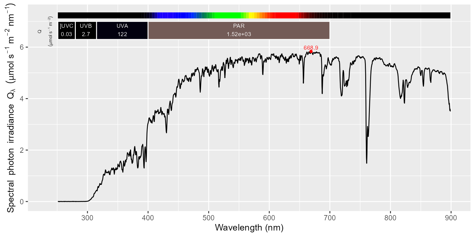
We can also use the same function to obtain counts per second. In other words linearising and dividing the raw counts by the integration time, splicing of spectra obtained using different integration times, applying the corrections inherent to the method selected and the wavelength calibration but not the calibration for the sensitivity of the pixels.
sun001_recalc.cps_spct <-
s_irrad_corrected(sun001.raw_mspct,
correction.method = ooacquire::MAYP11278_ylianttila.mthd,
return.cps = TRUE)## Warning: Dark spectrum failed QC: 209 hot, 6 cold pixelsAs the wavelength calibration is available for the whole wavelength
range, the returned spectrum expressed as counts per second includes all
the wavelengths acquired. In this cases this is an object of class
"cps_spct".
summary(sun001_recalc.cps_spct)## Summary of cps_spct [2,068 x 2] object: sun001_recalc.cps_spct
## Wavelength range 187.82-1117.14 nm, step 0.41-0.48 nm
## Label: light: sun001
## Measured on 2020-06-26 08:44:33.148438 UTC
## Data acquired with 'MayaPro2000' s.n. MAYP11278
## grating 'HC1', slit '010s'
## diffuser 'unknown'
## integ. time (s): 0.131, 1.31
## total time (s): 5.09, 5.22
## counts @ peak (% of max): 91.2
## w.length cps
## Min. : 187.8 Min. : -1261
## 1st Qu.: 431.7 1st Qu.: 40690
## Median : 668.7 Median :185474
## Mean : 663.3 Mean :201795
## 3rd Qu.: 897.6 3rd Qu.:364123
## Max. :1117.1 Max. :457476By plotting the raw counts expressed as counts per second we can see that the shape of the curve is affected by the varying sensitivity of the spectrometer to photons of different wavelengths.
autoplot(sun001_recalc.cps_spct)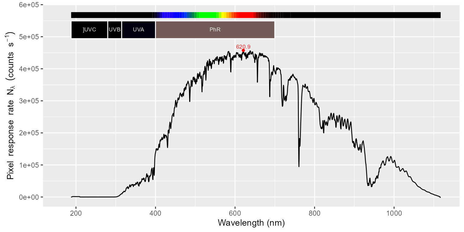
The instrument descriptor has been copied to
getInstrDesc(sun001_recalc.cps_spct)## Data acquired with 'MayaPro2000' s.n. MAYP11278
## grating 'HC1', slit '010s'
## diffuser 'unknown'Looking in more detail into this descriptor with
str().
str(getInstrDesc(sun001_recalc.cps_spct))## List of 16
## $ time : POSIXct[1:1], format: "2016-11-02 16:34:05"
## $ sr.index : int 0
## $ ch.index : int 0
## $ spectrometer.name: chr "MayaPro2000"
## $ spectrometer.sn : chr "MAYP11278"
## $ bench.grating : chr "HC1"
## $ bench.filter : chr "000"
## $ bench.slit : chr "010s"
## $ min.integ.time : int 7200
## $ max.integ.time : int 7200000
## $ max.counts : int 64000
## $ wavelengths : num [1:2068] 188 188 189 189 190 ...
## $ bad.pixs : num [1:6] 123 380 388 697 1829 ...
## $ inst.calib :List of 9
## ..$ nl.fun :function (x)
## .. ..- attr(*, "srcref")= 'srcref' int [1:8] 25 15 25 44 15 44 575 575
## .. .. ..- attr(*, "srcfile")=Classes 'srcfilealias', 'srcfile' <environment: 0x00000223ec347b38>
## ..$ straylight.coeff: num 0
## ..$ straylight.slope: num 0
## ..$ wl.fun :function (x)
## ..$ slit.fun : logi NA
## ..$ irrad.mult : num [1:2068] 0 0 0 0 0 0 0 0 0 0 ...
## ..$ wl.range : num [1:2] 251 899
## ..$ start.date : Date[1:1], format: "2018-04-01"
## ..$ end.date : Date[1:1], format: "2021-04-12"
## $ num.pixs : num 2068
## $ num.dark.pixs : num 20
## - attr(*, "class")= chr [1:2] "instr_desc" "list"We can in a separate step convert the counts per second data to
spectral irradiance by applying the calibration, which in this case is
available within sun001_recalc.cps_spct stored as a member
of the "intrument.desc" attribute.
sun001_recalc.source_spct <- cps2irrad(sun001_recalc.cps_spct)In this way we obtain the same irradiance spectrum as before.
summary(sun001_recalc.source_spct)
autoplot(sun001_recalc.source_spct)We can plot the calibration multipliers. The sensitivity of the pixels is lowest in the UV region, hence the multipliers are larger. The spectral energy is expressed per detector count (for a given cosine diffuser and fibre used). We obtain an irradiance when we multiply counts per second.
wavelengths <- getInstrDesc(sun001_recalc.cps_spct)$wavelengths
multipliers <- getInstrDesc(sun001_recalc.cps_spct)$inst.calib$irrad.mult
calib.spct <- calibration_spct(w.length = wavelengths,
irrad.mult = multipliers)
autoplot(calib.spct)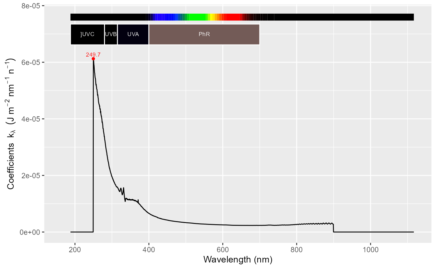
Step-by-step walk through
In this section we will apply one by one the different computation steps staring from RAW spectral data until we obtain spectral irradiance, ´to obtain the same spectrum shown in the figure above. Unless mentioned explicitly all the steps in this walk-through apply to all the methods described above.
We have described in the previous section the structure of the object containing the RAW counts data. As we saw above, measurements consisted in two measurements using two different integration times. In addition to different integration times, the number of “scans” was adjusted so that each of the two spectra contain data for a similar total length of time. This averaging takes place before the data are “seen” by R. The three spectra, light, filter and dark where acquired one after another and using the same settings in the spectrometer.
When dealing with raw detector counts one needs to be aware that the array detector in array spectrometers saturates at a certain number of counts, ranging from 256 to 65000 or more counts (e.g., 64000 counts in the Maya 2000 Pro as shown here and fewer simpler/older models like the USB2000). This information is stored as part of the metadata.
getInstrDesc(sun001.raw_mspct[["light"]])$max.counts## [1] 64000If more photons imping on a detector cell/pixel during one integration event (or “scan”) than needed to reach 64000 counts, the reading remains at 64000 counts. This is usually called “signal clipping”, i.e., the tips of peaks are truncated or off scale.
We can find out what integration times have been used from the metadata stored in the same object. In the example spectrum, the shorter integration time used was near optimal, avoiding clipping but still using more the 90% of the pixel counts at the peak. However, the light source has also regions with low emission so we also used a 10 times longer integration time, resulting in clipping of peaks, but making better use of the sensor in the “darker” parts of the spectrum. By changing the number of individual integrations averaged, the total accumulated duration of the measurement was kept at approximately 5 s.
getInstrSettings(sun001.raw_mspct[["light"]])## integ. time (s): 0.131, 1.31
## total time (s): 5.09, 5.22
## counts @ peak (% of max): 91.2Plotting the two bracketed spectra shows the effect of using the two
different integration times (counts_1 is the average of 39
integrations each 0.131 s-long, and counts_2 is the average
of 4 integration each 1.31 s-long). Note: The first four pixels in each
spectrum are “dark” pixels that are not exposed to light, i.e., the
counts are smaller than for other pixels and similar for the short and
long integration times. These will show in the plots of the raw spectra
as a clear dip in the curve. A similar, but unexpected, dip can be seen
at the other end in the infrared.
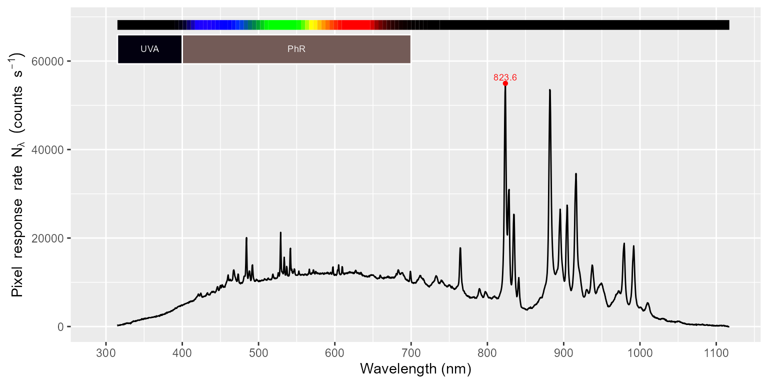
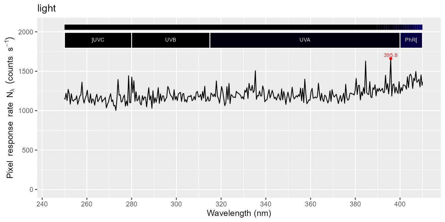
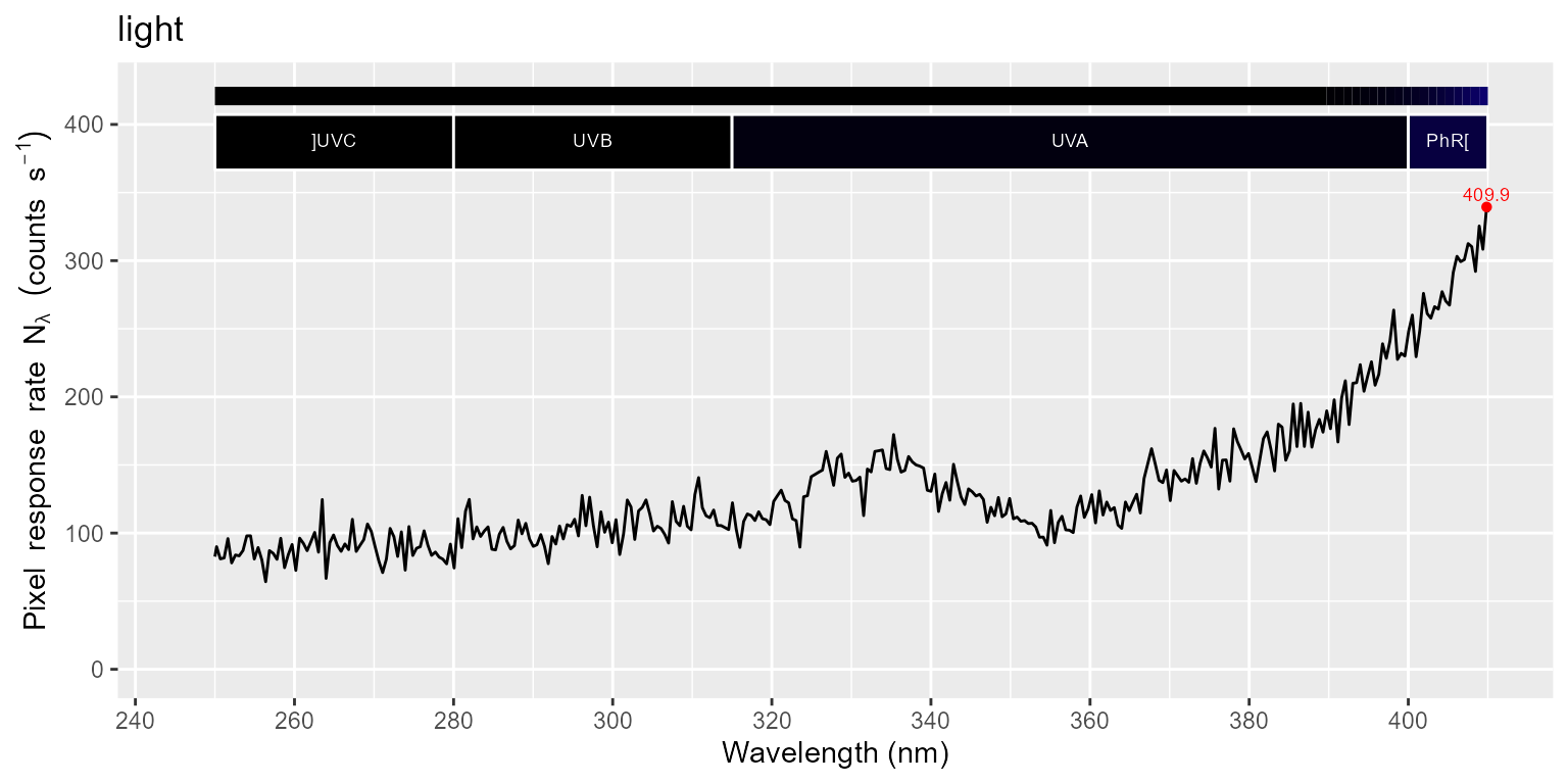
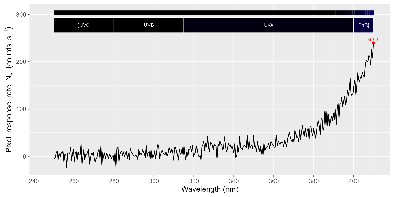
autoplot(sun001.raw_mspct[["light"]])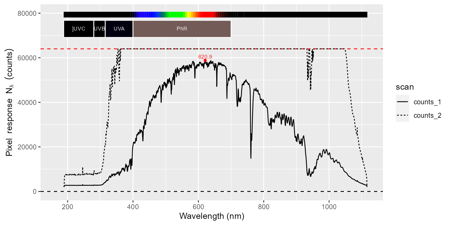
In the figure above, we can see that in addition to clipping, increasing the integration time, at least in some spectrometers, significantly increases the “noise floor” or dark readings. This is also true for the measurements done in darkness. In these spectra, we can also easily see several spikes caused by “hot pixels” in the detector (over-responding pixels). In the figure below we can see the effect of the filter.
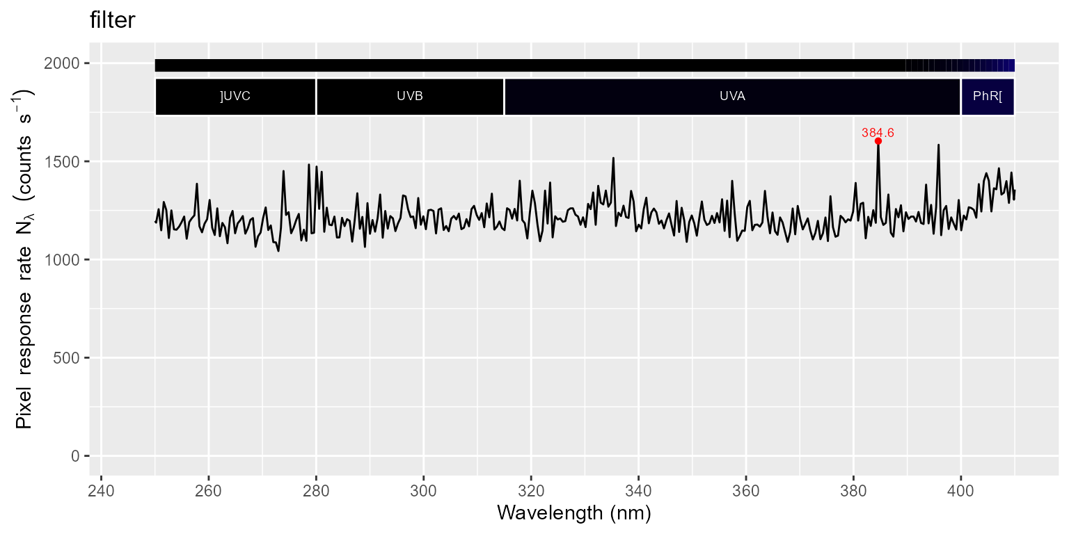
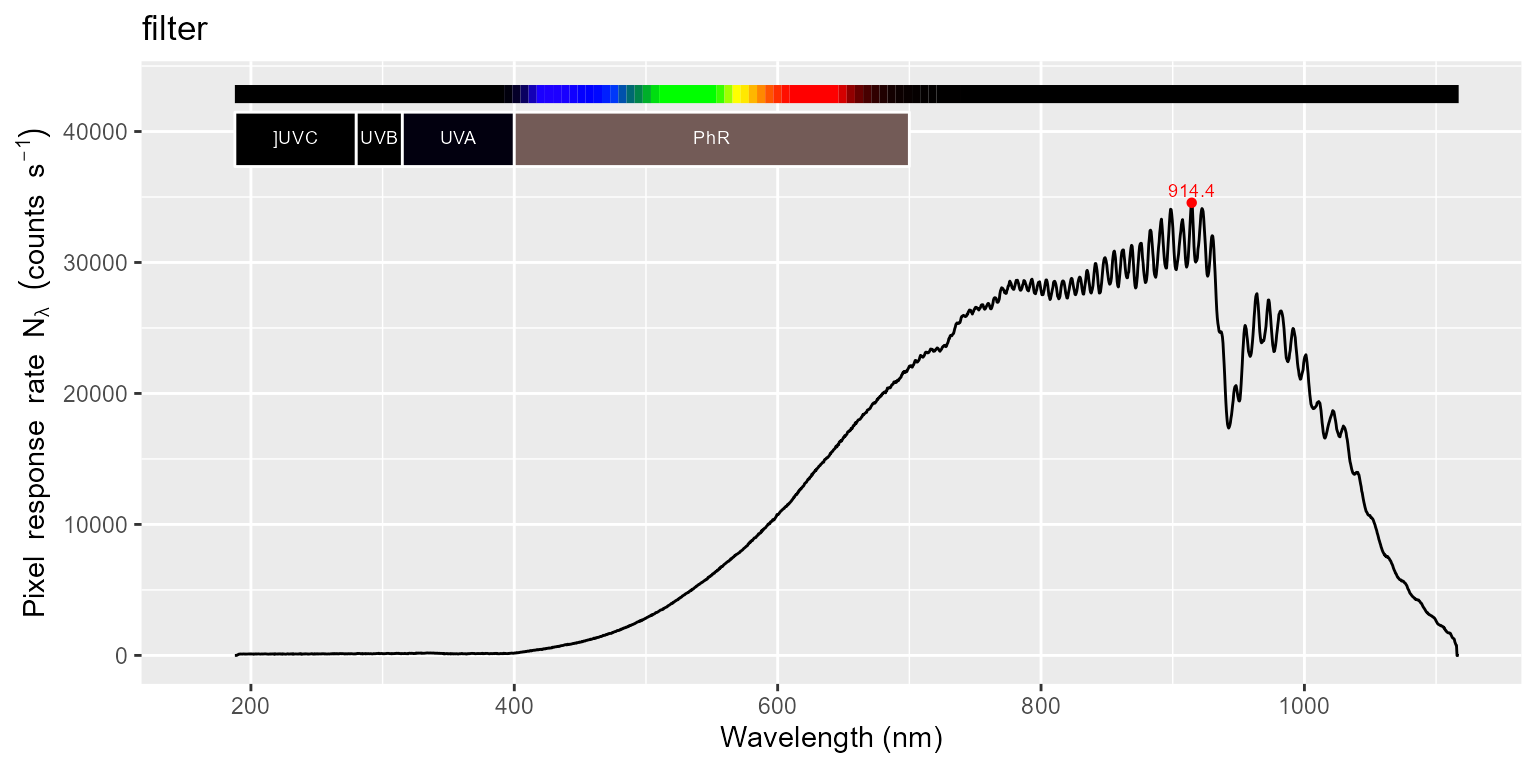
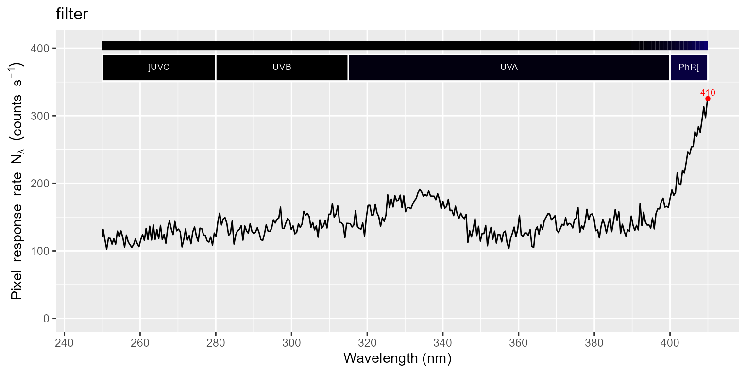
autoplot(sun001.raw_mspct[["filter"]])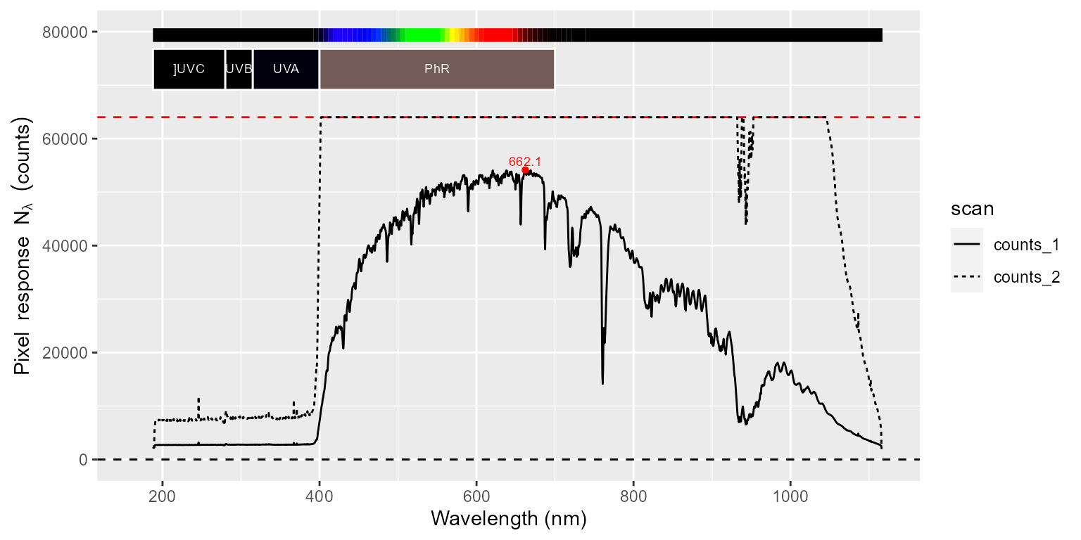
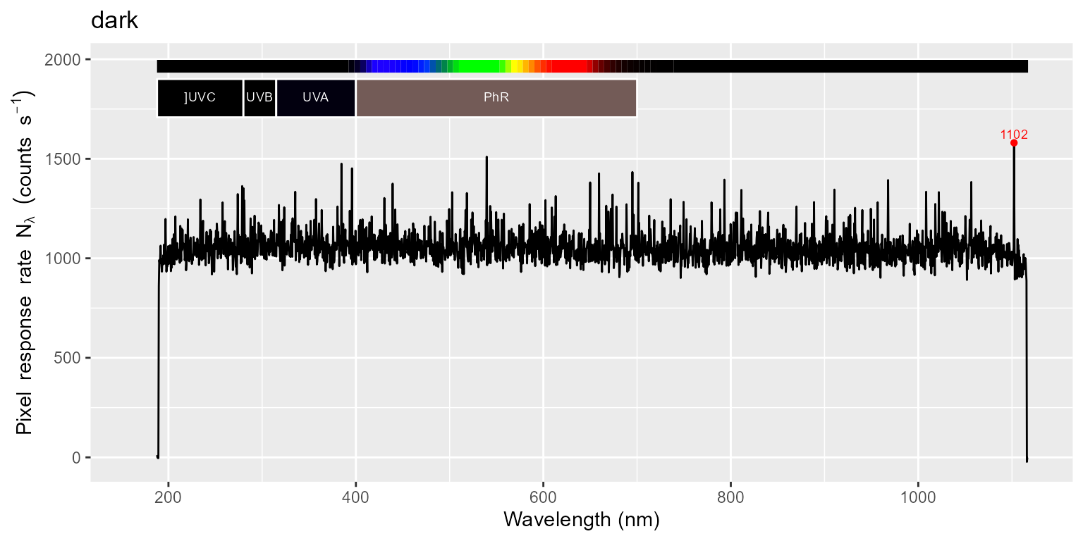
In this third figure, we have a look at the spectrum measured in darkness. The Maya 2000 Pro spectrometer has the peculiarity that the effect of warming on dark noise depends on wavelength.
autoplot(sun001.raw_mspct[["dark"]])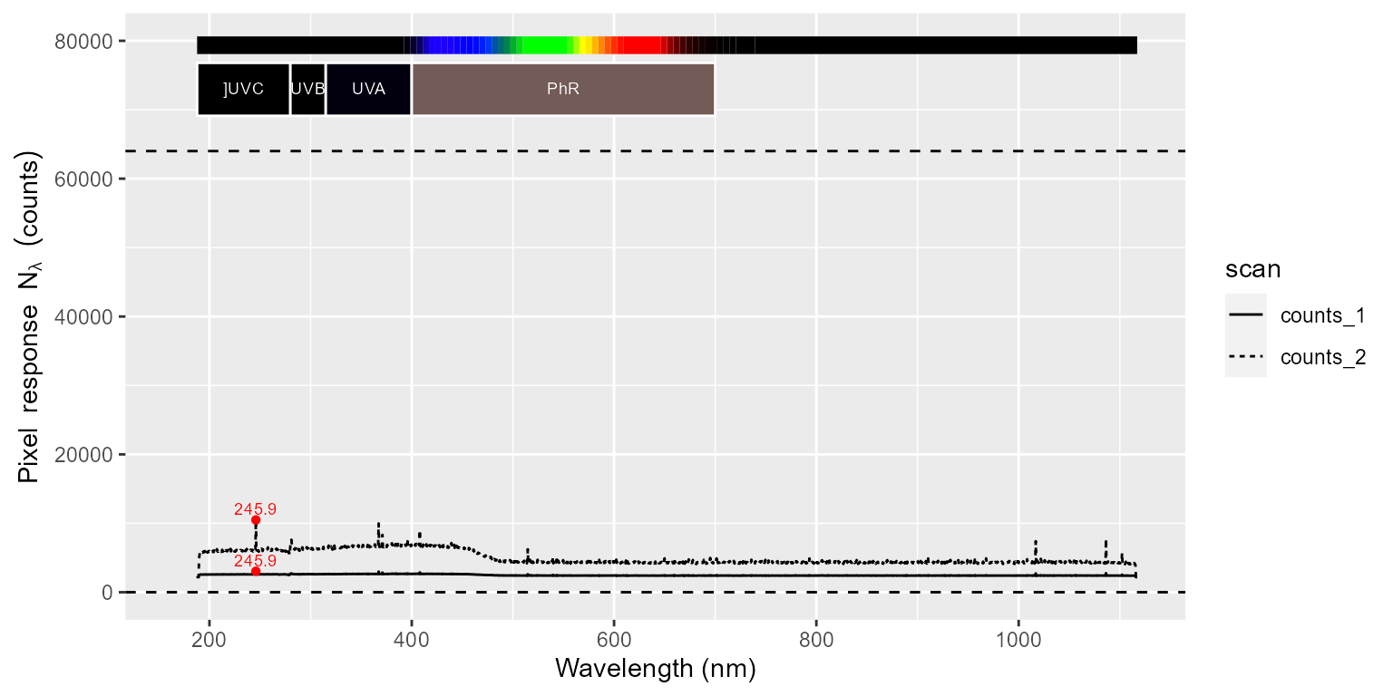
The first step in the processing is to substitute data from known bad pixels by values interpolated from the adjacent fixels. Which pixels are bad is recorded in the calibration data. What this step achieves can be clearly seen by comparing the plots before (see above) and after this step (see below). As in most array spectrometers pixel resolution is better than optical resolution this introduces little error, except possibly in the case of very narrow peaks.
for (m in names(sun001.raw_mspct)) {
sun001.raw_mspct[[m]] <-
skip_bad_pixs(sun001.raw_mspct[[m]])
}
autoplot(sun001.raw_mspct, facets = 1)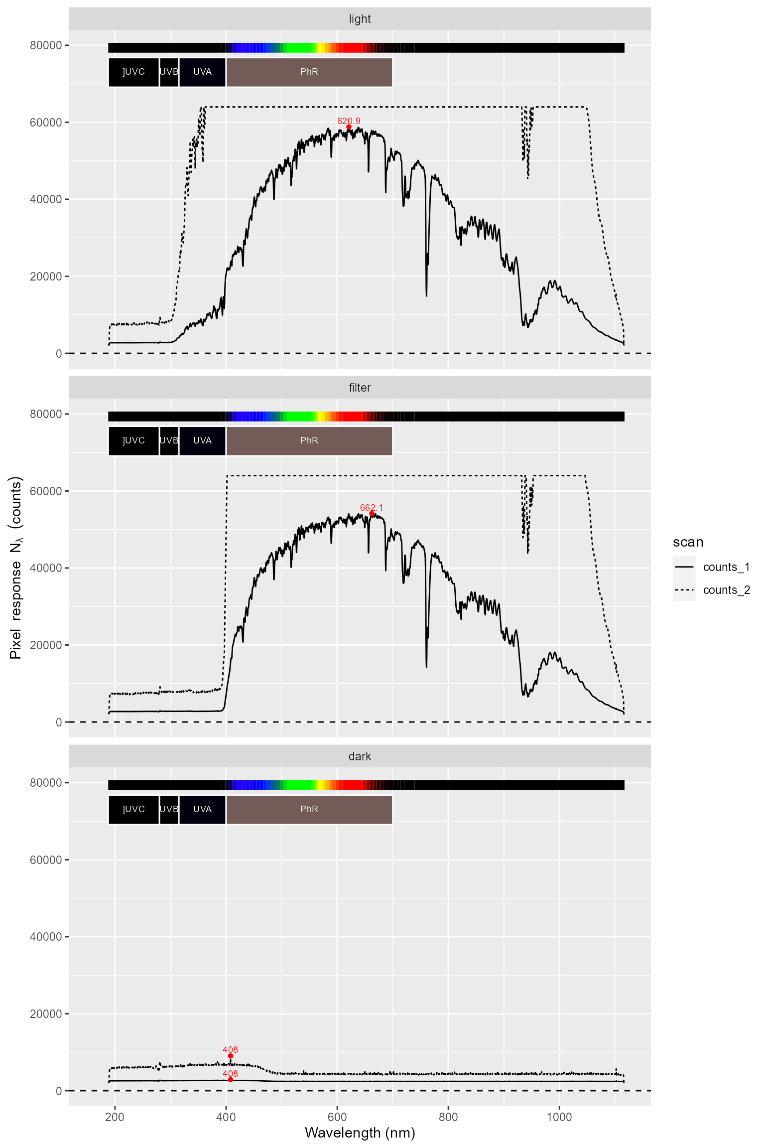
Note: When bad-pixel information is not available, automatic despiking can be used instead, but it needs care not to accidentally remove true peaks from the data. (In some types of measurements the spikes appear randomly as they are triggered by cosmic high-energy particles making use of a despiking algorithm a necessity.)
The second step is to replace saturated (clipped)
pixel data, with the missing data marker NA. As
NA values are not plotted pixels exactly equal to the
maximum possible reading disappear from the plots.
for (m in names(sun001.raw_mspct)) {
sun001.raw_mspct[[m]] <-
trim_counts(sun001.raw_mspct[[m]])
}
autoplot(sun001.raw_mspct, facets = 1)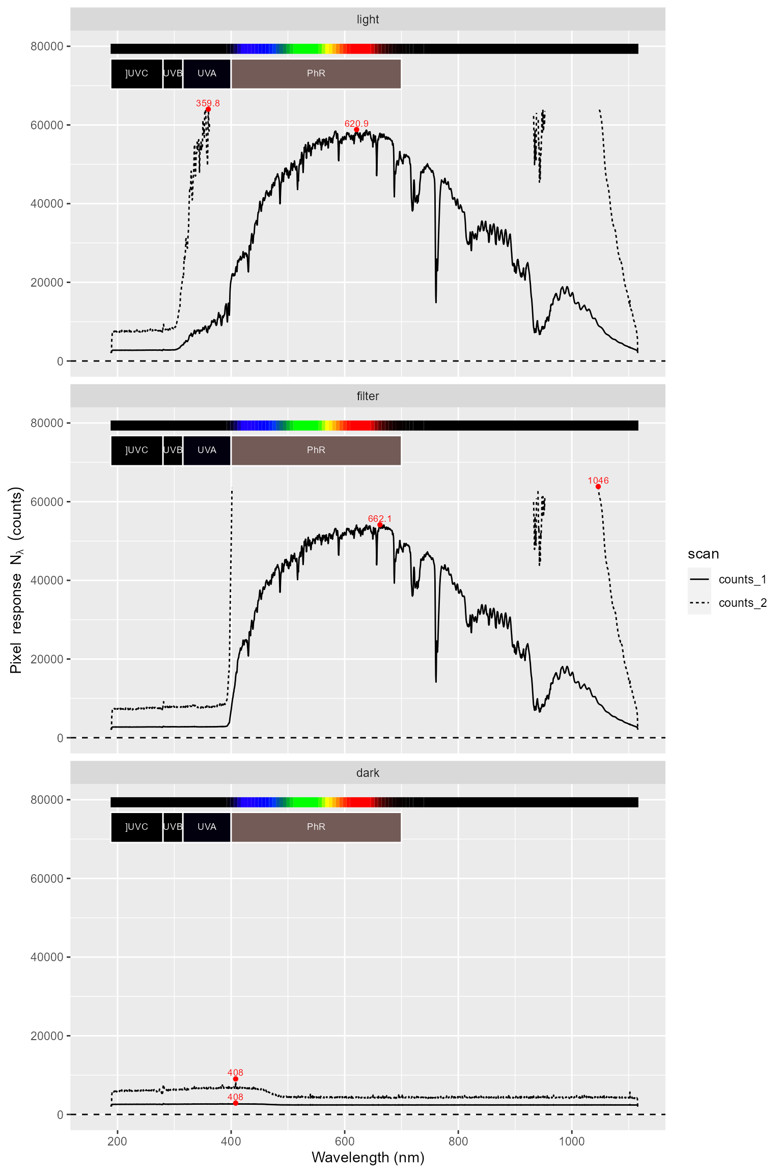
An important consideration is that when a pixel well fills
with electrical charge some of the excess charge migrates to nearby
pixels. How many nearby pixels are affected depends on the detector
type, but it is at most a few tens of pixels. So in this third
step, pixels neighbouring those set to NA in the
second step are also set to NA. By default we replace the
values from the 10 nearest neighbouring non-saturated pixels also by
NA.
for (m in names(sun001.raw_mspct)) {
sun001.raw_mspct[[m]] <-
bleed_nas(sun001.raw_mspct[[m]])
}
autoplot(sun001.raw_mspct, facets = 1)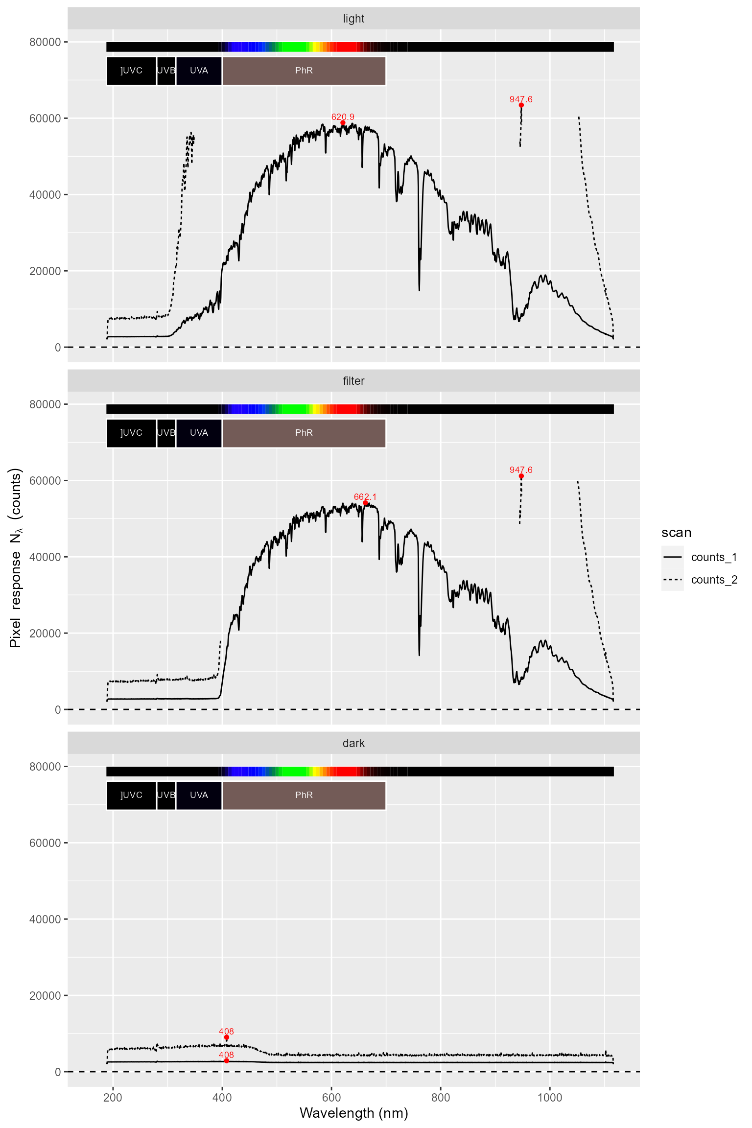
The response of array detectors is not perfectly linear to the number of photons received. Most precisely when the number of counts gets near the maximum value, the sensitivity to additional photons slightly decreases. This is a result of how “full” the sensor wells are, irrespective of the source of the charge (on-target light, stray light or thermal energy). Consequently this correction should be applied before subtraction of the dark reading.
So, the fourth step is to apply a linearisation function, in most cases supplied with the instrument and possibly stored in the instrument firmware. This function is part of the calibration data for the instrument that is stored as metadata during acquisition of the spectra. Given that linearization corrects for a decrease in sensitivity at counts approaching the maximum, some values can exceed the maximum instrument counts once corrected (> 64000 in our case).
for (m in names(sun001.raw_mspct)) {
sun001.raw_mspct[[m]] <-
linearize_counts(sun001.raw_mspct[[m]])
}
autoplot(sun001.raw_mspct, facets = 1)
The first few pixels in the detector of most array spectrometers are covered and never exposed to light photons. These can be used as a dark reference to correct for thermal noise. This step may appear redundant, but might help in cases when instrument temperature is not the same during the light and dark measurements. An alternative is to use pixels known not to be exposed to radiation from the light source, but within the useful measurement range of the instrument. Sunlight at ground level is known to lack UV-C photons, so wavelengths between 250 nm and 290 nm can used as dark reference for this light source. Consequently, as the fifth step we remove an estimate of dark signal based on “non-excited pixels”. As seen in the plots, this step effectively removes the overall dark signal from both light and dark measurements. We can, however, also see that there is residual dark noise remaining at pixel level, not all pixels have the same noise floor. Part of this variation is systematic, and some may be random. As we used a total measurement time of 5 s much of the random noise must have cancelled out through averaging.
for (m in names(sun001.raw_mspct)) {
sun001.raw_mspct[[m]] <-
fshift(sun001.raw_mspct[[m]], range = c(218.5,228.5))
}
autoplot(sun001.raw_mspct, facets = 1)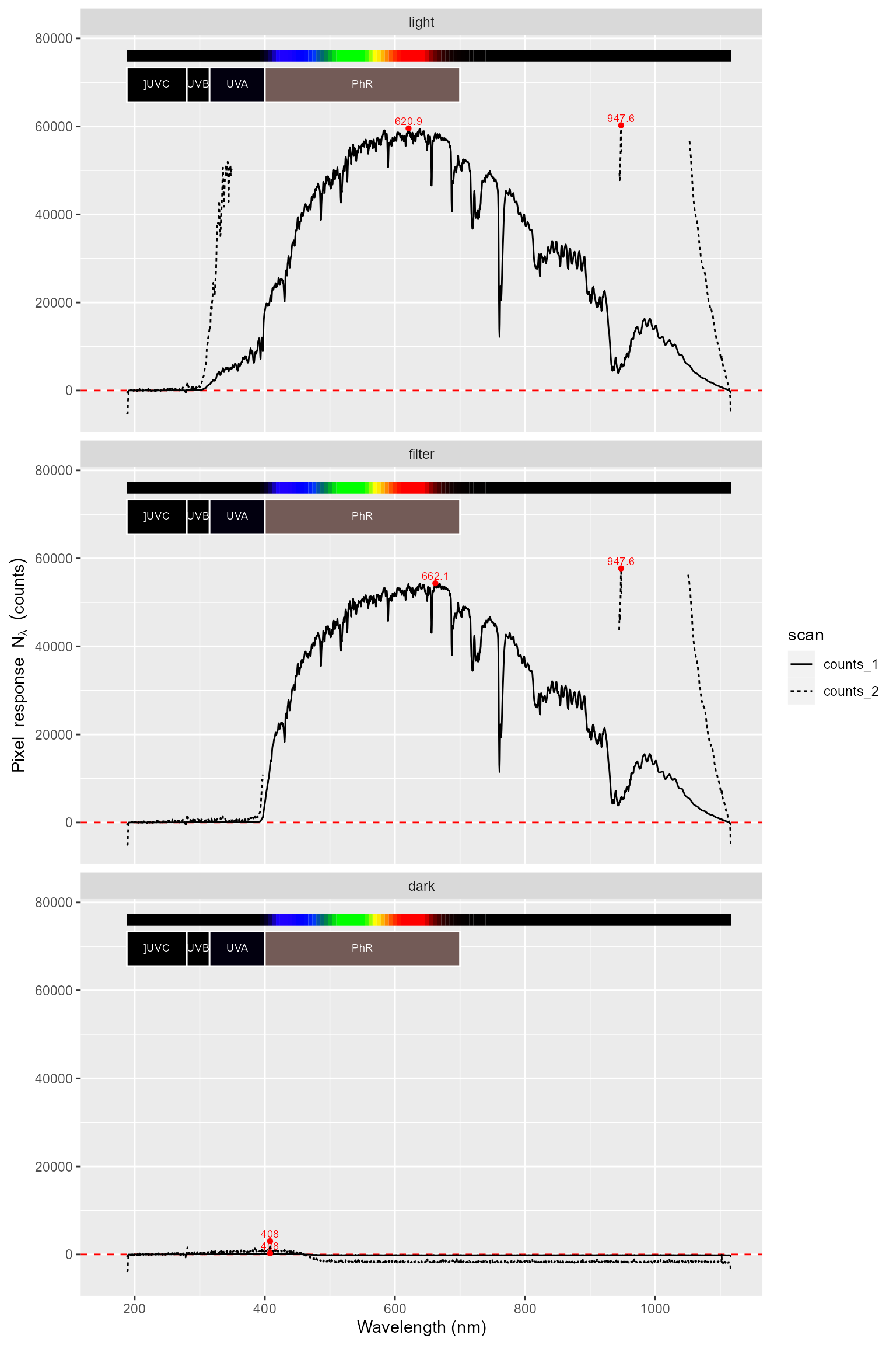
In the last plot above we can see that the correction has resulted in slightly negative values in darkness. If the bump in the noise floor, caused by warming, is consistent among all three measurements, it will cancel out.
At this point we have “clean” RAW counts data. The sixth
step is to convert these raw counts into counts per second. As
the integration time for each spectrum is stored together with the RAW
count data, the function call is simple. After this step, the data
acquired using different integration times are expressed in the same
units of counts-per-second (cps or \(n\,s^{-1}\)). We take advantage of this to
plot using different colours the data from the two different “bracketed”
integration times. Blue corresponds to the shorter and near-optimal
integration time (cps_1 computed starting from
counts_1), and red to the longer one (cps_2
computed starting from counts_2). Here we over-plot the two
separate spectra.
sun001.cps_mspct <- raw2cps(sun001.raw_mspct)## Warning in range_check(x, cps.cols): Possible off-range cps values
## [-3069.27..2255.09]
## Warning in range_check(x, cps.cols): Possible off-range cps values
## [-3069.27..2255.09]## Warning in range_check(x, cps.cols): Possible off-range cps values
## [-2954.70..2314.79]
# autoplot(sun001.cps_mspct, facets = TRUE)The seventh step splicing the three pairs of “bracketed” light, filter and dark counts-per-second spectra into three combined spectra.
## Warning in range_check(x, cps.cols): Possible off-range cps values
## [-2954.70..2314.79]
autoplot(sun001.cps_mspct)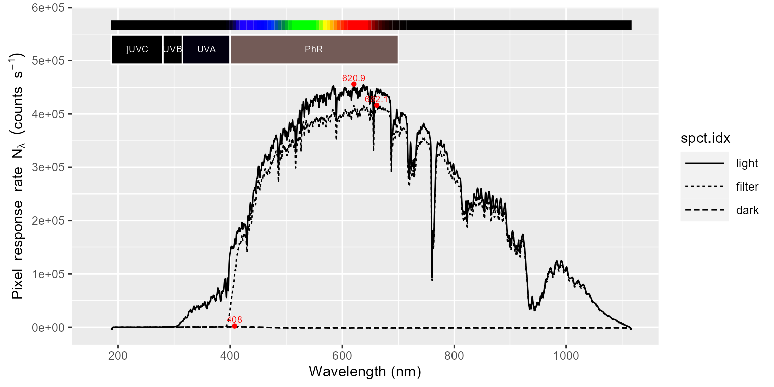
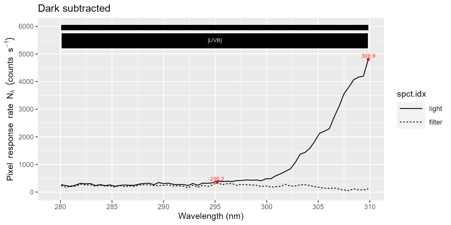
In the eighth step we subtract the dark signal from the light and filter measurements. This reduces the remaining noise. The filter used has a rather sharp cut-in very close to 400 nm, and blocks UV radiation from entering the spectrometer, so the UV signal remaining after subtracting the dark measurement is the result of light of wavelengths longer than 400 nm “wrongly” striking the UV pixels in the array, i.e., stray light.
In first plot below it looks like there is no stray light present, but zooming-in into the UV-B region we can see that stray light makes a significant contribution to the readings at these short wavelengths.
sun001_mdark.cps_mspct <- cps_mspct()
sun001_mdark.cps_mspct[["light"]] <-
sun001.cps_mspct[["light"]] - sun001.cps_mspct[["dark"]]
sun001_mdark.cps_mspct[["filter"]] <-
sun001.cps_mspct[["filter"]] - sun001.cps_mspct[["dark"]]
sun001_mdark.cps_mspct[["dark"]] <- NULL
autoplot(sun001_mdark.cps_mspct) + ggtitle("Dark subtracted")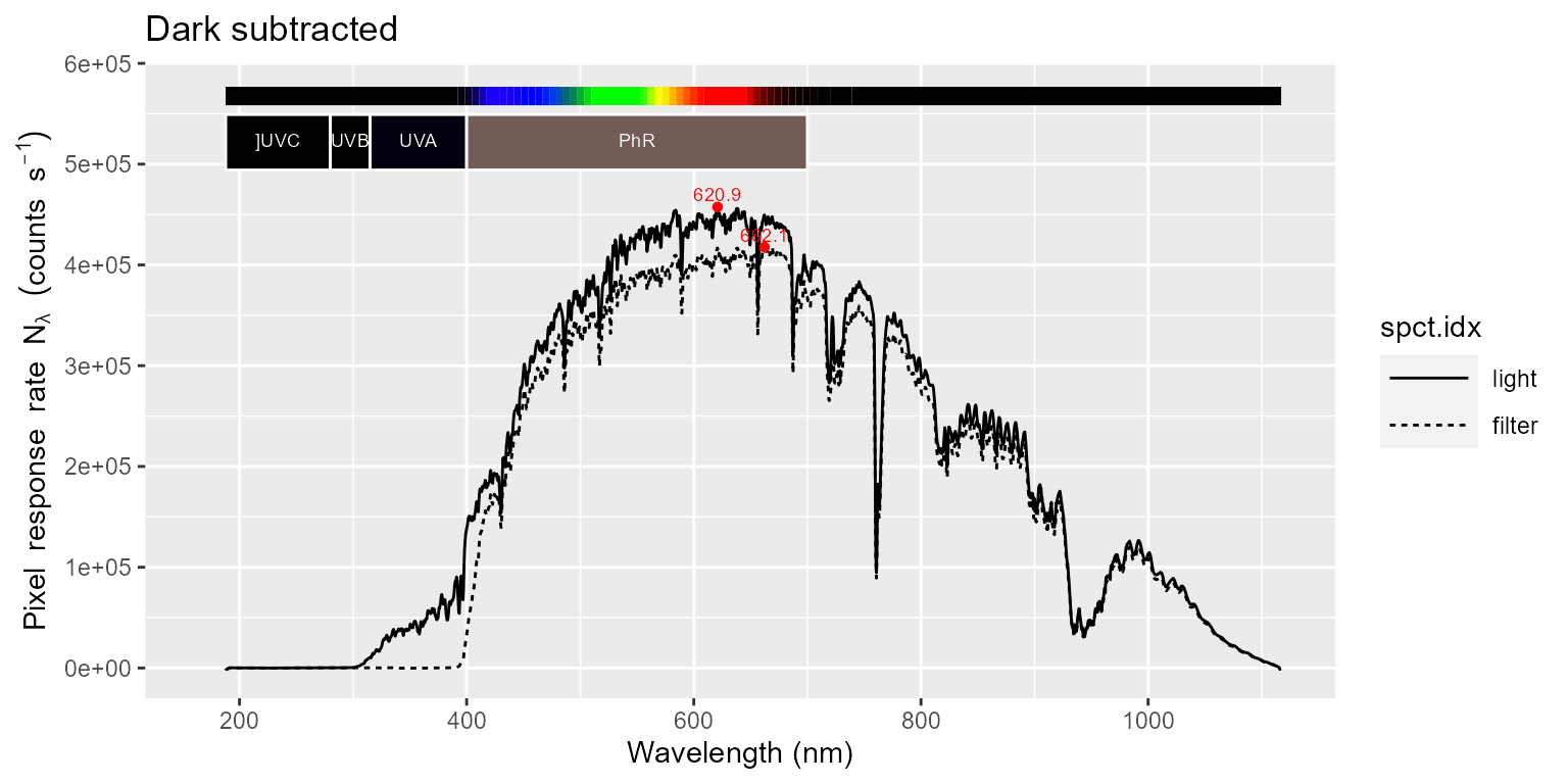
To further assess the approximate contribution of stray light to the readings we plot the ratio between these two spectra. Considering that the filter transmits only about 85% of the stray light, we can see that as expected there is only stray light at wavelengths < 293 nm. The methods also estimate absorption of stray light by the filter from the data itself. This estimate also includes and compensates for variation in incident irradiance between light and filter measurements. (However, it does not compensate for changes in the shape of the spectrum of the incident light between light and filter measurements.)
ggplot(clip_wl(sun001_mdark.cps_mspct[["filter"]] /
sun001_mdark.cps_mspct[["light"]],
range = c(280, 310))) +
geom_line() +
geom_hline(yintercept = 0.85, linetype = "dotted") +
ggtitle("Stray light contribution to cps") +
labs(y = "Contribution of stray light to readings (/1)",
x = "Waavelength (nm)")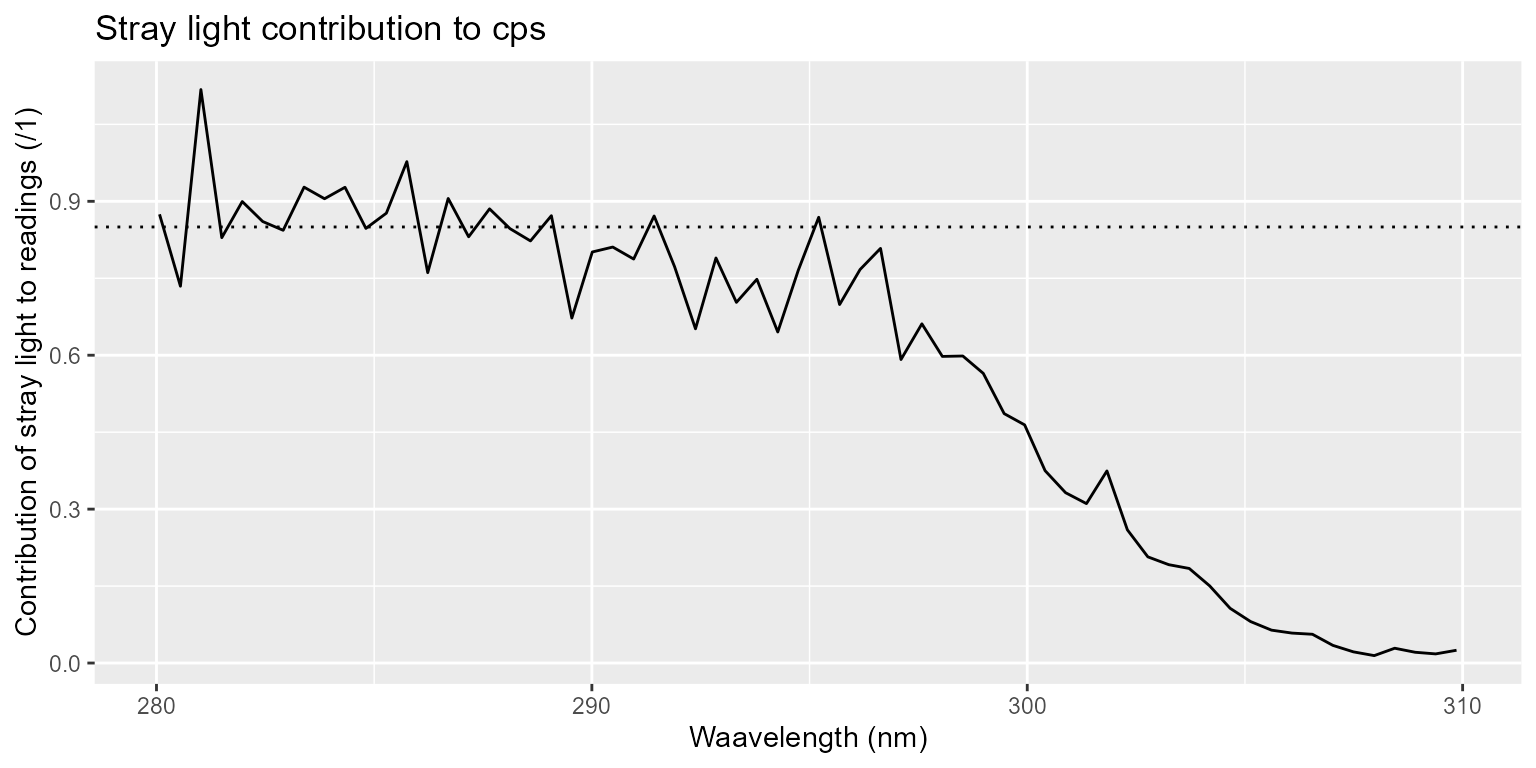
At this point we have a clean counts-per-second spectrum. However, as we have used math operators on the data, we need to restore the metadata.
sun001_mdark.cps_mspct[["light"]] <-
copy_attributes(sun001.cps_mspct[["light"]],
sun001_mdark.cps_mspct[["light"]])
sun001_mdark.cps_mspct[["filter"]] <-
copy_attributes(sun001.cps_mspct[["filter"]],
sun001_mdark.cps_mspct[["filter"]])The ninth step is to apply the calibration
multipliers and any additional instrument specific correction to obtain
spectral irradiance stored in a "source_spct" object.
We first demonstrate how the light measurement with no stray
light correction and the filter measurement look like when
plotted. This light spectrum is equivalent to using method
none. The ratio between the UV-C reading and PAR is close
to \(3 \times 10^{-4}\) in this case.
For sunlight this ratio is usally near \(1
\times 10^{-3}\).
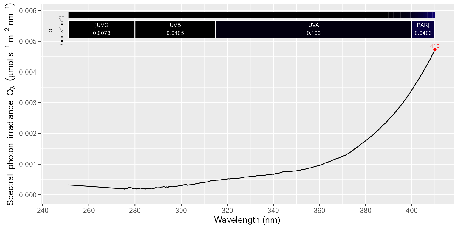
sun001.irrad_spct <- cps2irrad(sun001_mdark.cps_mspct[["light"]])
autoplot(sun001.irrad_spct)
sun001_filter.irrad_spct <- cps2irrad(sun001_mdark.cps_mspct[["filter"]])
autoplot(sun001_filter.irrad_spct)In an optional, step we apply smoothing to remove some of the noise from the light spectrum, but although the UV-C and UV-B regions look cleaner the value of the summaries remain unchanged and affected by stray light.
sun001.irrad_spct <- smooth_spct(sun001.irrad_spct)
autoplot(sun001.irrad_spct)One key aspect of the more sophisticated methods, is the stray light
correction. We here replot the spectrum obtained using method
ylianttila or original. We can see that UV-C
is less than \(3 \times 10^{-5}\)
compared to PAR, and the estimate of UV-B has decreased by 13%. The
estimates for UV-A and PAR irradiances remain unchanged.
autoplot(sun001_recalc.spct)
We can also apply smoothing to this spectrum, which in this case improves even further the UV-C estimate, which is now less than \(5 \times 10^{-6}\) which is an exceptionally good performance, which is rarely achieved for this method, with a usual ratio close to \(1 \times 10^{-4}\). So, by using Ylianttila’s method we have improved the signal to noise ratio by more than an order of magnitude.
autoplot(smooth_spct(sun001_recalc.spct))Before continuing with a different example we explain how the stray
light correction is done in method Ylianttila or
original. The exact wavelengths used in the algorithm are
tuned for each individual spectrometer and are part of the method.
str(MAYP11278_ylianttila.mthd)## List of 10
## $ spectrometer.sn : chr "MAYP11278"
## $ stray.light.method: chr "original"
## $ stray.light.wl : num [1:2] 218 228
## $ flt.dark.wl : num [1:2] 193 210
## $ flt.ref.wl : num [1:2] 360 380
## $ flt.Tfr : num 1
## $ inst.dark.pixs : int [1:3] 2 3 4
## $ tail.coeffs : num [1:2] -7.2731 -0.0569
## $ worker.fun : chr "MAYP11278_tail_correction"
## $ trim : num 0We have three ranges of wavelengths. For sunlight we can assume that
pixels for wavelengths in flt.ref.wl have received enough
photons to be very little affected by stray light.
flt.dark.wl is the range of wavelengths where we assume the
filter is fully opaque. stray.light.wl is a wavelength
range where we can safely assume (for sunlight) that both light
and filter measurement are just pure stray light; thus, these
pixels can be used to rescale the filter measurement to
compensate for filter transmittance less than one for stray light or
changes in stray light caused by a change in incident irardiance. This
assumes thay stray light is scattered rather than due to specular
reflections within the spectrometer.
ADD DETAILS OF CORRECTION METHODS
Obviosuly, this filter-based correction, as implemented in
correction methos original are applicable only to
measurements of sunlight or of spectra very similar in shape to
sunlight, like natural shade light.
With a LED source that does not emit in the IR, at least in the case of our Maya 2000 Pro, we do not need to worry about stray light. However, when we measure light sources with a significant emission in the infra-red above 900 nm, stray light becomes a problem. In addition sources with narrow peaks of emission may benefit from deconvolution or correction based on a measurement of the slit function.
Tungsten halogen lamp
For our instrument, stray light originates mostly in the infra-red and it can be a serious problem when trying to precisely measuring sunlight or incandescent lamps. For this example we use data acquired using a different protocol, which includes three measurements, being the additional one, a measurement through a filter used to estimate stray light in the UV-region. In this case a UV-cut and IR-pass filter (a piece of clear polycarbonate).
The data contains a measurement of the light source directly and through a filter and a reference dark measurement.
names(halogen.raw_mspct)## [1] "light" "filter" "dark"The spectrum for the light measurement contains two columns with RAW-counts data.
names(halogen.raw_mspct[["light"]])## [1] "w.length" "counts_1" "counts_2"Summary in addition to displaying the summary for the columns, displays the most important metadata attributes.
summary(halogen.raw_mspct[["light"]])## Summary of raw_spct [2,068 x 3] object: anonymous
## Wavelength range 187.82-1117.14 nm, step 0.41-0.48 nm
## Label: Halogen
## Measured on 2017-03-28 11:24:35.664327 UTC
## Data acquired with 'MayaPro2000' s.n. MAYP11278
## grating 'HC1', slit '010s'
## diffuser 'unknown'
## integ. time (s): 1.86, 7.2
## total time (s): 5.58, 7.2
## counts @ peak (% of max): 94.4
## w.length counts_1 counts_2
## Min. : 187.8 Min. : 2121 Min. : 1950
## 1st Qu.: 431.7 1st Qu.: 5316 1st Qu.:14164
## Median : 668.7 Median :22588 Median :64000
## Mean : 663.3 Mean :25981 Mean :44225
## 3rd Qu.: 897.6 3rd Qu.:44996 3rd Qu.:64000
## Max. :1117.1 Max. :60728 Max. :64000As above for the LED lamp, we first calculate spectral irradiance
from a set of raw-counts spectral data using the high-level function
s_irrad_corrected().
halogen.spct <-
  s_irrad_corrected(halogen.raw_mspct, correction.method= MAYP11278_ylianttila.mthd)
autoplot(halogen.spct)
In the example above we called the functions used for each of the steps in the computation individually, saving the intermediate results so as to be able to show the partly processed data at each step. The functions, however, support the use of pipes as they all have as their first parameter the one accepting the R object returned by the previous stage.
We first use a “pipe” to apply the same initial processing steps as for the LED bulb data in the previous section. The main difference is that we use as internal instrument dark reference those pixels that never are exposed to radiation. For our instrument they correspond to wavelengths 187.82 nm to 189.26 nm. We obtain this time three spectra containing counts-per-second data.
halogen.cps_mspct <- cps_mspct()
for (m in names(halogen.raw_mspct)) {
  halogen.raw_mspct[[m]] %>%
    skip_bad_pixs() %>%
    trim_counts() %>%
    bleed_nas() %>%
    linearize_counts() %>%
    fshift(range = c(187.82,189.26)) %>%
    raw2cps() %>%
    merge_cps() -> halogen.cps_mspct[[m]]
}
names(halogen.cps_mspct)
## [1] "light" "filter" "dark"We plot the returned spectra, both in full, and the UV region by itself. Please, be aware of the difference in the y scale among the plots. By careful comparison of these later plots one can see that the signal for filter is larger than for dark. As we know from specifications and measurements that the filter used blocks radiation in this region, the difference is due to stray light (radiation of longer wavelengths being detected as ultraviolet).
for (m in names(halogen.cps_mspct)) {
  print(autoplot(halogen.cps_mspct[[m]]) + ggtitle(m))
  print(autoplot(halogen.cps_mspct[[m]], range = c(250, 410)) + ggtitle(m))
}

In the next step we subtract the dark reading from both the light and filter readings, and copy attributes, including instrument settings and calibration data.
halogen01.cps_mspct <- cps_mspct()
for (m in setdiff(names(halogen.cps_mspct), "dark")) {
  halogen01.cps_mspct[[m]] <- halogen.cps_mspct[[m]] - halogen.cps_mspct[["dark"]]
  halogen01.cps_mspct[[m]] <-
    copy_attributes(halogen.cps_mspct[[m]],
                    halogen01.cps_mspct[[m]],
                    copy.class = FALSE)
}
names(halogen01.cps_mspct)
## [1] "light" "filter"The second and fourth plots display in detail the UV region. Be aware of the difference in the y scale in the plots
for (m in names(halogen01.cps_mspct)) {
  print(autoplot(halogen01.cps_mspct[[m]]) + ggtitle(m))
  print(autoplot(halogen01.cps_mspct[[m]], range = c(250, 410)) + ggtitle(m))
}
As we can see in the plots above, a small amount of stray light is
present in both spectra in the UV region. We apply a filter correction
using a simple method based on a fixed transmittance value. We set
flt.Tfr = 0.9 as these is a good estimate of the
transmittance of polycarbonate to the stray light.
halogen_corrected.cps_spct <-
  filter_correction(halogen01.cps_mspct[["light"]],
                    halogen01.cps_mspct[["filter"]],
                    stray.light.method = "original",
                    flt.Tfr = 0.9)
names(halogen_corrected.cps_spct)
## [1] "w.length" "cps"
getTimeUnit(halogen_corrected.cps_spct)## [1] "second"The second plot displays in detail the UV region. Be aware of the difference in the y scale in the plots
autoplot(halogen_corrected.cps_spct)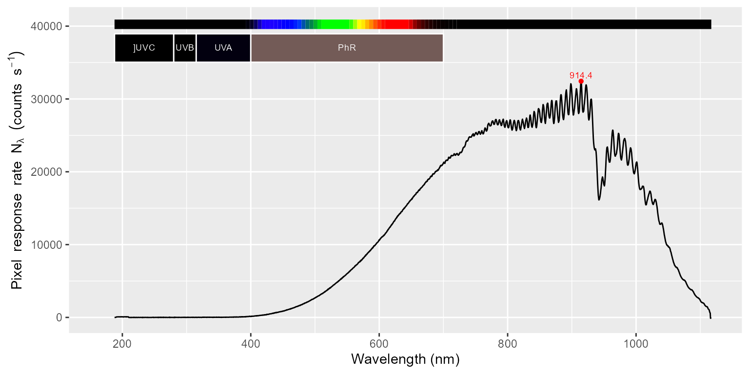
## [1] 2.747068The average counts-per-second remaining after correcting for stray light is very small. In the next step we apply the calibration multipliers to obtain spectral irradiance.
## [1] "w.length" "s.e.irrad"The spectrum displays some noise at the shortest wavelengths and some interference patterns at the long end. The interference patterns come from the light bulb, but the random noise of increasing amplitude with decreasing wavelength in the UV region is due to the spectrometer.
We can compute some photon ratios, expressed as \(mmol\, mol^{-1}\) to diagnose whether the stray light is well controlled.
## ]UVC:PAR[q:q]  UVB:PAR[q:q]  UVA:PAR[q:q]
##     0.1925562     0.3494061     3.2901570
## attr(,"radiation.unit")
## [1] "q:q ratio"
Smoothing can sometimes help, but it can also introduce bias. It should be used with care and always checking the output.
Using defaults, we get some minor artifacts in the UV region, but preserve the data pattern in the NIR.
halogen_sm0.source_spct <- smooth_spct(halogen.source_spct)## 368 possibly 'bad' values in smoothed spectral responseThe second plot displays in detail the UV region. Be aware of the difference in the y scale in the plots
autoplot(halogen_sm0.source_spct)
How much difference did smoothing do?
## ]UVC:PAR[q:q]  UVB:PAR[q:q]  UVA:PAR[q:q]
##    0.00000000    0.09519497    3.07102788
## attr(,"radiation.unit")
## [1] "q:q ratio"
With overriding the default arguments we better remove random noise
and a small “bump” at 320 nm. Setting setting strength to
1 instead of 3 smooths the random noise but
not this small peak (not shown). In the infra-red most of the wavy
pattern is also removed. So, smoothing can be useful, but it can also
remove real features, and one needs to decide if these features are of
interest or not, based on other sources of information.
halogen_sm.source_spct <- smooth_spct(halogen.source_spct, method = "supsmu", strength = 3)The second plot displays in detail the UV region. Be aware of the difference in the y scale in the plots: the ratio between the irradiance at 280 nm and at 900 nm is 1:3500.
autoplot(halogen_sm.source_spct)
How much difference did smoothing do?
## ]UVC:PAR[q:q]  UVB:PAR[q:q]  UVA:PAR[q:q]
##     0.2395183     0.3434062     3.4877545
## attr(,"radiation.unit")
## [1] "q:q ratio"
Slit function correction
When measuring spectra containing narrow peaks or steep slopes the shape of the slit function will affect the apparent width of peaks or the apparent steepness of the slope. The slit through which light enters the instrument has a finite width and angle of acceptance for radiation. Consequently, even when measuring true monochromatic radiation from a laser photons will imping on multiple array pixels/wells. The pixel corresponding to the wavelength of the radiation receives the most photons, but the neighbouring pixels receive a decreasing number of photons as the distance from the “correct” target pixel increases. The wider the slit used, the broader the “false” peak observed for monochromatic light. The shape and width of this slit function depends not only on the width of the slit but also on other features of the optical bench of the instrument. In array spectrometers the slit function also depends on wavelength as the length of the path from the grating to the detector is not constant.
However, if the slit function is known, it can be used to remove its influence from a measured spectrum, in simpler words it can be used to partly reconstruct the structure of original light source spectrum. In the case of the two examples above, applying this correction would make little difference. In the case of the solar spectrum and discharge lamps this further step improves the estimates for spectral irradiance.
Too see the effect of this correction we need to look at individual peaks in a spectrum. We use data for a mercury lamp.
The data contains a measurement of the light source and a reference dark measurement.
names(xenon_flash.raw_mspct)## [1] "light" "dark"The spectrum for the light measurement contains one column with RAW-counts data as no bracketing was used.
names(xenon_flash.raw_mspct[["light"]])## [1] "w.length" "counts"Summary in addition to displaying the summary for the columns, displays the most important metadata attributes.
summary(xenon_flash.raw_mspct[["light"]])## Summary of raw_spct [2,068 x 2] object: anonymous
## Wavelength range 187.82-1117.14 nm, step 0.41-0.48 nm
## Label: Bare bulb xenon flash
## Measured on 2018-09-13 14:34:06.442208 UTC
## Data acquired with 'MayaPro2000' s.n. MAYP11278
## grating 'HC1', slit '010s'
## diffuser 'unknown'
## integ. time (s): 5.08
## total time (s): 5.08
## counts @ peak (% of max): 91.9
## w.length counts
## Min. : 187.8 Min. : 2096
## 1st Qu.: 431.7 1st Qu.: 8150
## Median : 668.7 Median :13992
## Mean : 663.3 Mean :13795
## 3rd Qu.: 897.6 3rd Qu.:17637
## Max. :1117.1 Max. :57992In the case of these data, the concept of counts-per-second does not apply as the flash discharge is shorter than the integration time, and unknown. The relevant reference is one exposure event and the quantity to estimate is spectral fluence in \(J m^{-2}\).
getInstrSettings(xenon_flash.raw_mspct[["light"]])$num.exposures## [1] 1As above for the LED lamp, we first calculate spectral fluence from a
set of raw-counts spectral data using the high-level function
s_irrad_corrected().
xenon_flash.spct <-
  s_irrad_corrected(xenon_flash.raw_mspct, correction.method = MAYP11278_ylianttila.mthd)
getTimeUnit(xenon_flash.spct)
## [1] "exposure"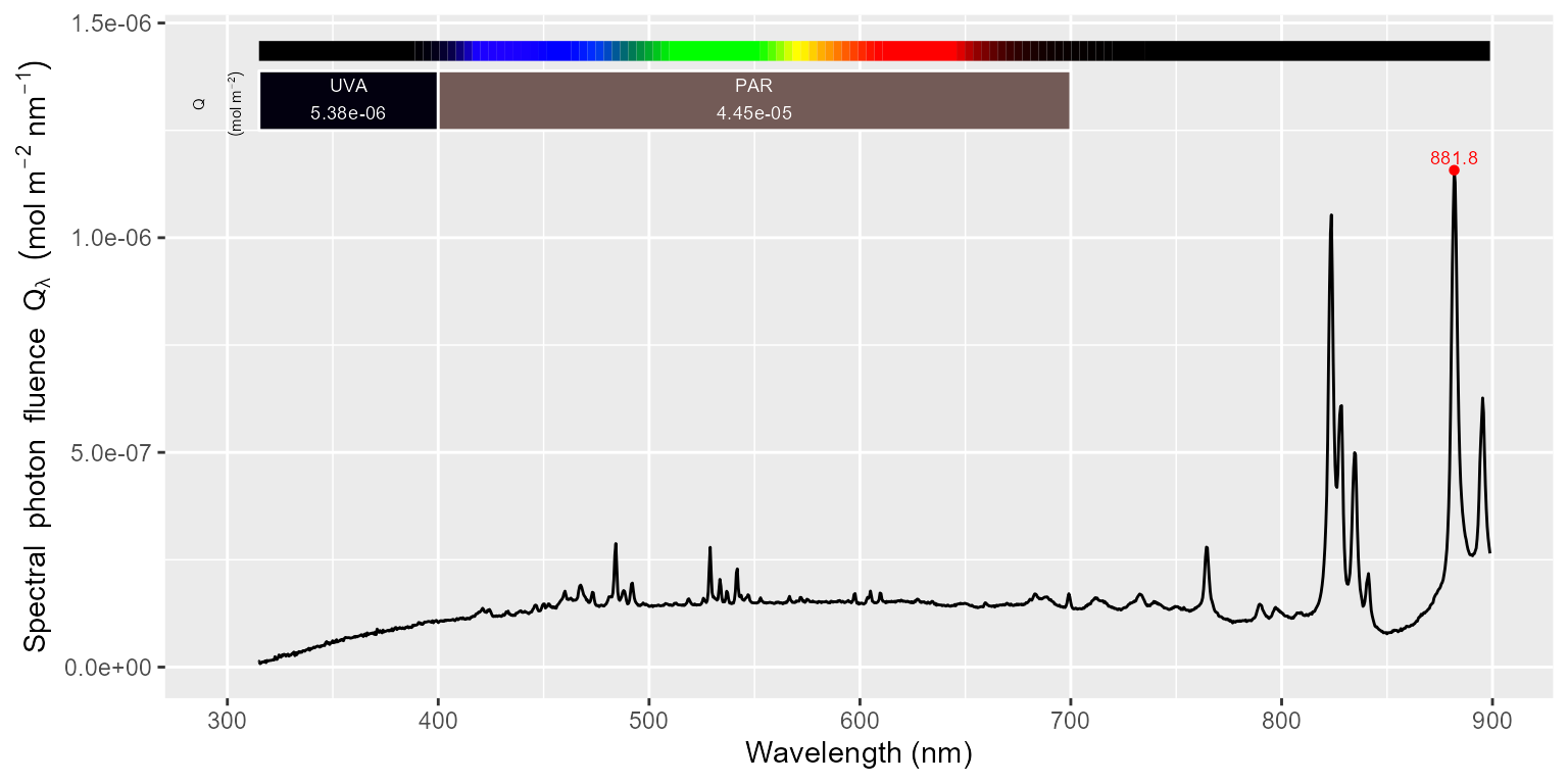
xenon_flash.cps_spct <-
  s_irrad_corrected(xenon_flash.raw_mspct, correction.method= MAYP11278_ylianttila.mthd, return.cps = TRUE)
getTimeUnit(xenon_flash.cps_spct)
## [1] "exposure"