User Guide

Introduction

This package provides data sets and functions relevant to the photobiology of plants. It is part of a suite, which has package ‘photobiology’ at its core. Please visit (http://www.r4photobiology.info/) for more details. For more details on plotting spectra, please consult the documentation for package ‘ggspectra’, and for information on the calculation of summaries and maths operations between spectra, please, consult the documentation for package ‘photobiology’.

See the User Guide for packages ‘photobiology’ and ‘ggspectra’ for instructions on how to work with spectral data. As package ‘ggspectra’ is only suggested, in this vignette it is loaded an used conditionally on its availability.

library(photobiology)
library(photobiologyPlants)
library(photobiologyWavebands)
eval_plots <- requireNamespace("ggspectra", quietly = TRUE)
if (eval_plots) library(ggspectra)

theme_set(theme_bw())

Light environment

Photon ratios

R_FR() and other functions for computing photon ratios are convenience functions implemented using function q_ratio() and q_irrad() from package ‘photobiology’ and waveband definitions from package ‘photobiologyWavebands’ with defaults arguments to parameter std for wavelength ranges commonly used in the field of plant photobiology. These functions can be used with one or more spectra as argument.

R_FR(sun.spct)

## R:FR[q:q] 
##  1.242474 
## attr(,"radiation.unit")
## [1] "q:q ratio"

Here, the argument named attr2tb is forwarded to method q_ratio from package ‘photobiology’ to copy metadata from the spectra into the returned data frame.

R_FR(sun_evening.spct, 
     std = "Smith20", 
     attr2tb = c("when.measured" = "time.UTC", "lat" = "latitude"))

## # A tibble: 5 × 4
##   spct.idx `R:FR[q:q]` time.UTC            latitude
##   <fct>          <dbl> <dttm>                 <dbl>
## 1 time.01         1.18 2023-06-12 18:38:00     60.2
## 2 time.02         1.19 2023-06-12 18:39:00     60.2
## 3 time.03         1.18 2023-06-12 18:40:00     60.2
## 4 time.04         1.16 2023-06-12 18:41:00     60.2
## 5 time.05         1.12 2023-06-12 18:42:00     60.2

Photoreceptors

Phytochromes: photoequilibrium

In the examples below we use the solar spectral data included in package ‘photobiology’ as a data frame in object sun.spct.

We can calculate the phytochrome photoequilibrium from spectral irradiance data contained in a source_spct object as follows.

Pfr_Ptot(sun.spct)

## [1] 0.68341

We can also calcualte the red:far-red photon ratio, in this second example, for the same spectrum as above

R_FR(sun.spct)

## R:FR[q:q] 
##  1.242474 
## attr(,"radiation.unit")
## [1] "q:q ratio"

which is equivalent to calculating it using package ‘photobiology’ directly

q_ratio(sun.spct, Red("Smith10"), Far_red("Smith10"))

## R:FR[q:q] 
##  1.266704 
## attr(,"radiation.unit")
## [1] "q:q ratio"

We can, and should whenever spectral data are available, calculate the photoequilibrium as above, directly from these data. It is possible to obtain and approximation in case of the solar spectrum and other broad spectra, using the red:far-red photon ratio. The calculation, however, is only strictly valid, for di-chromatic illumination with red plus far-red light.

Pfr_Ptot_R_FR(R_FR(sun.spct))

## R:FR[q:q] 
## 0.7025925

Here we calculated the R:FR ratio from spectral data, but in practice one would use this function only when spectral data is not available as when a R plus FR sensor is used. We can see that in such a case the photoequilibrium calculated is only a rough approximation. For sunlight, in the example above when using spectral data we obtained a value of 0.683 in contrast to 0.703 when using the R:FR photon ratio. For other light sources differences can be much larger. Furthermore, here we used the true R:FR ratio calculated from the spectrum, while broad-band red:far-red sensors guive only an approximation, which is good for sunlight, but which will be innacurate for artifical light, unless a special calibration is done for each type of lamp.

In the case of monochromatic light we can still use the same functions, as the defaults are such that we can use a single value as the ‘w.length’ argument, to obtain the Pfr:P ratio. For monochromatic light, irradiance is irrelevant for the photoequilibrium (steady-state).

Pfr_Ptot(660)

## [1] 0.869649

Pfr_Ptot(735)

## [1] 0.01749967

Pfr_Ptot(c(660, 735))

## [1] 0.86964902 0.01749967

Pfr_Ptot(435)

## [1] 0.3859998

We can also plot Pfr:Ptot as a function of wavelength (nm) of monochromatic light. The default is to return a vector for short input vectors, and a response_spct object otherwise, but this can be changed through argument spct.out.

autoplot(Pfr_Ptot(300:770), unit.out = "photon",
         w.band = Plant_bands(),
         annotations = c("colour.guide", "labels", "boxes")) +
  labs(y = "Phytochrome photoequilibrium, Pfr:Ptot ratio")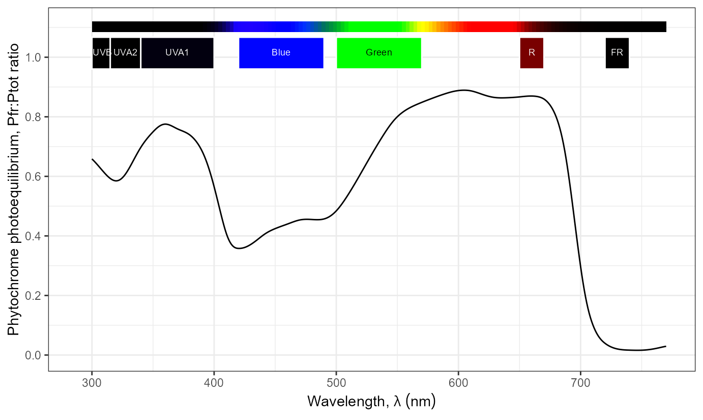

It is, of course, also possible to use base R plotting functions, or as shown here functions from package ‘ggplot2’

ggplot(data = Pfr_Ptot(300:770), aes(w.length, s.q.response)) +
  geom_line() +
  labs(x = "Wavelength (nm)",
       y = "Phytochrome photoequilibrium, Pfr:Ptot ratio")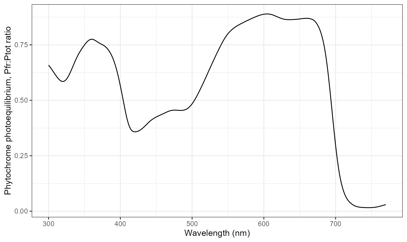

In the case of dichromatic illumination with red (660 nm) and far-red (730 nm) light, we can use a different function that takes the R:FR photon ratio as argument.

These computations are valid only for true mixes of light at these two wavelengths but not valid for broad spectra like sunlight and especially inaccurate for plant growth lamps with peaks in their output spectrum, such as most discharge lamps (sodium, mercury, multi-metal, fluorescent tubes) and many LED lamps.

Pfr_Ptot_R_FR(1.15)

## [1] 0.6919699

Pfr_Ptot_R_FR(0.01)

## [1] 0.04747996

Pfr_Ptot_R_FR(c(1.15,0.01))

## [1] 0.69196990 0.04747996

It is also easy to plot Pfr:P ratio as a function of R:FR photon ratio. However we have to remember that such values are exact only for dichromatic light, and only a very rough approximation for wide-spectrum light sources. For wide-spectrum light sources, the photoequilibrium should, if possible, be calculated from spectral irradiance data.

ex6.data <- data.frame(r.fr=seq(0.01, 5.0, length.out=100), Pfr.p=numeric(100))
ex6.data$Pfr.p <- Pfr_Ptot_R_FR(ex6.data$r.fr)
ggplot(data=ex6.data, aes(r.fr, Pfr.p)) +
  geom_line() +
    labs(x ="R:FR photon ratio",
         y = "Phytochrome photoequilibrium, Pfr:Ptot ratio")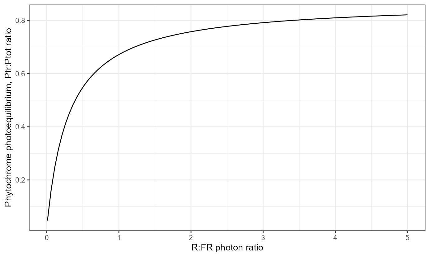

Phytochromes: reaction rates

with(clip_wl(sun.spct, c(300,770)), Phy_reaction_rates(w.length, s.e.irrad))

## $k1
## [1] 1.25935
## 
## $k2
## [1] 0.5833947
## 
## $nu
## [1] 1.842745

Phytochromes: absorption cross section at given wavelengths

The phytochrome photoequilibrium cannot be calculated from the absorptance spectra of Pr and Pfr, because Pr and Pfr have different quantum yields for the respective phototransformations. We need to use action spectra, which in this context are usually called absorption cross-sections'. They can be calculated as the product of absorptance and quantum yield. The values in these spectra, in the case of Phy are calledSigma’.

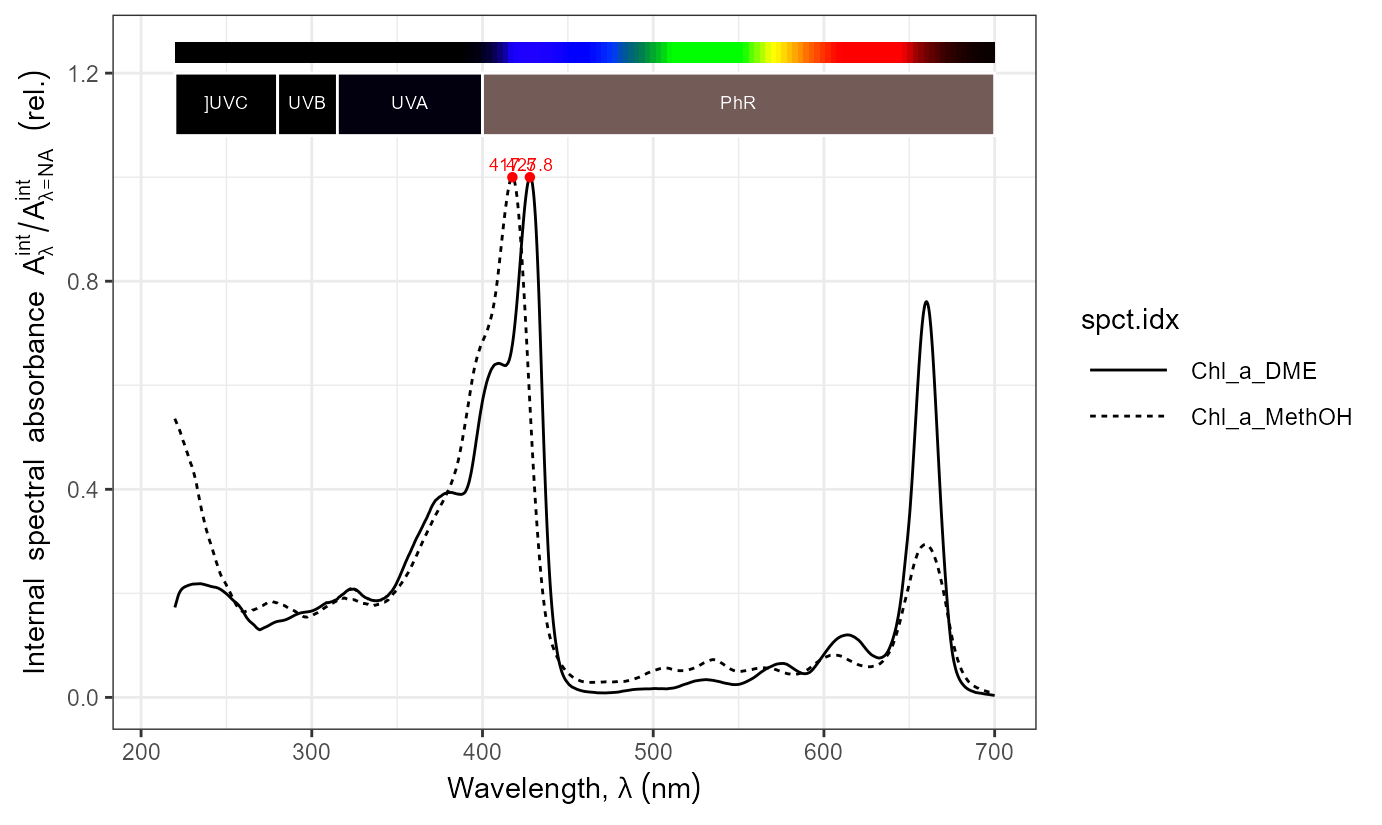
Here we reproduce Figure 3 in Mancinelli (1994), which gives the ‘Relative photoconversion cross-sections’ of Pr (\sigma_R) and Pfr (\sigma_{FR}). The values are expressed relative to \sigma_R at its maximum at \lambda = 666 nm.

ex7.data <- data.frame(w.length=seq(300, 770, length.out=100))
ex7.data$sigma.r <- Phy_Sigma_R(ex7.data$w.length)
ex7.data$sigma.fr <- Phy_Sigma_FR(ex7.data$w.length)
ex7.data$sigma <- Phy_Sigma(ex7.data$w.length)
ggplot(ex7.data, aes(x = w.length)) +
  geom_line(aes(y = sigma.r/ max(sigma.r)), colour = "red") +
  geom_line(aes(y = sigma.fr/ max(sigma.r))) +
  labs(x = "Wavelength (nm)", y = expression(sigma[R]~"and"~sigma[FR]))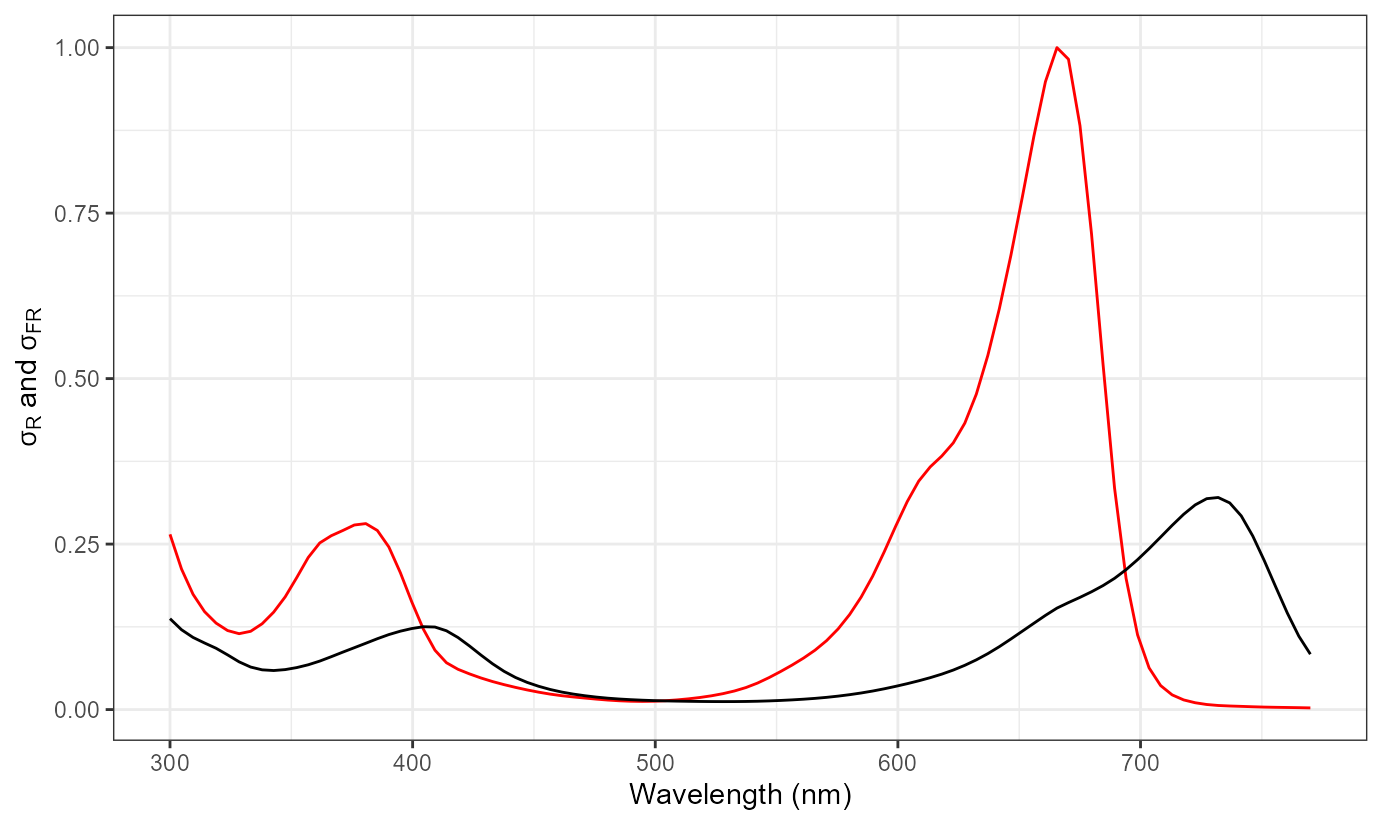

rm(ex7.data)

Cryptochromes: spectral absorbance

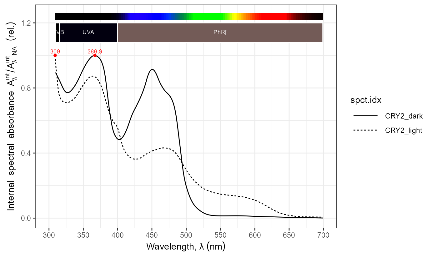
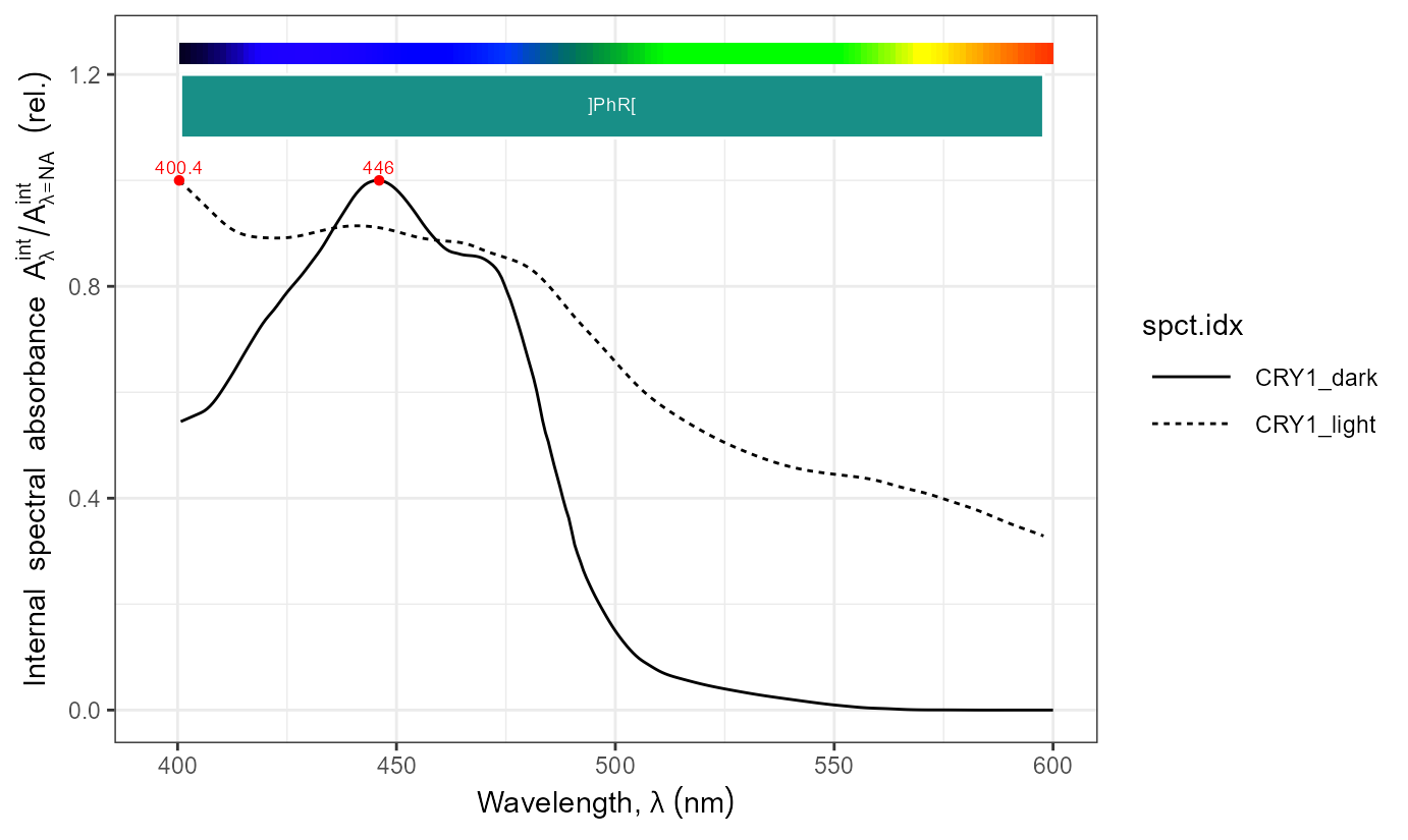
names(CRYs.mspct)

## [1] "CRY1_dark"  "CRY1_light" "CRY2_dark"  "CRY2_light" "CRY3_dark"

Here we approximate Figure 1.B from Banerjee et al. (2007).

A_as_default()
autoplot(CRYs.mspct$CRY2_dark)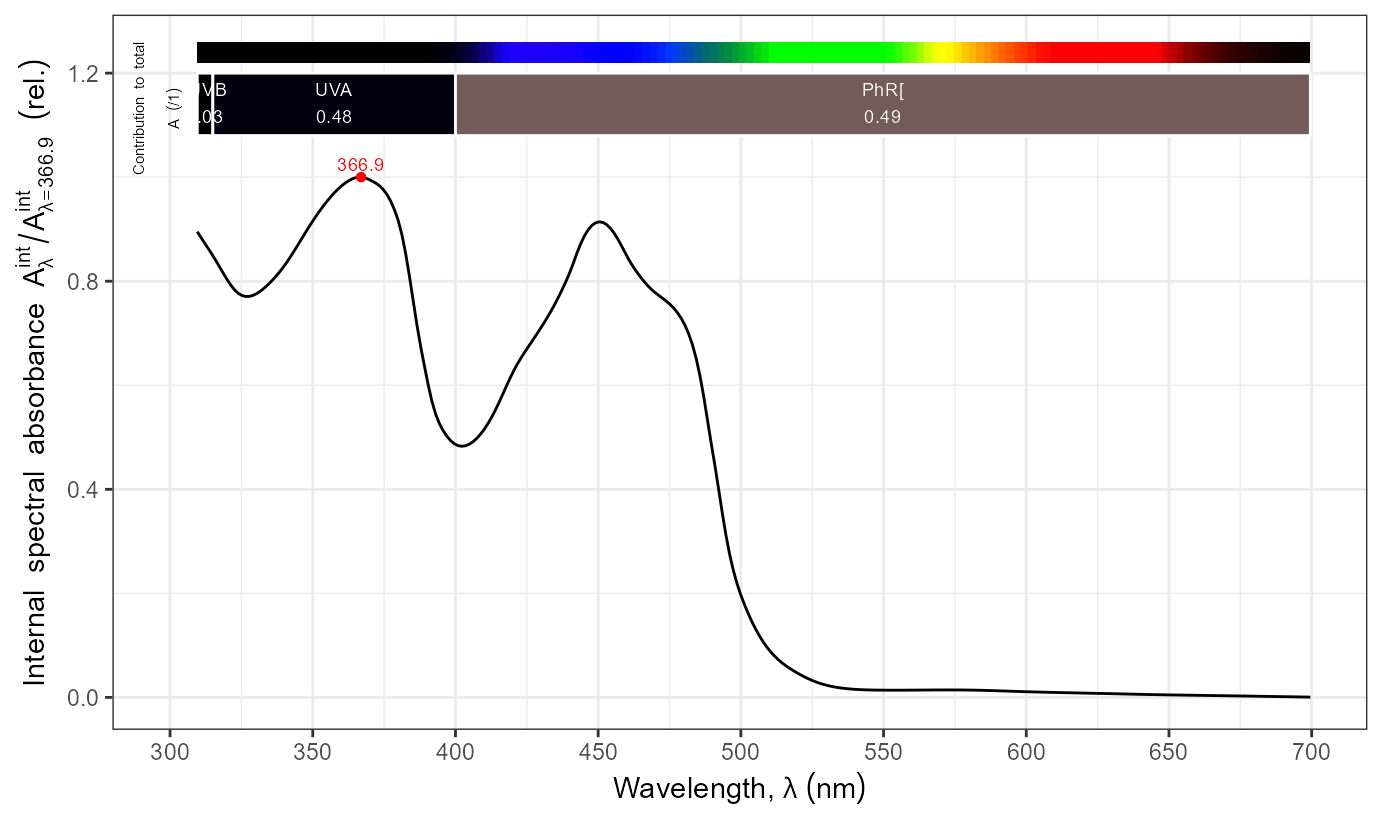

autoplot(CRYs.mspct[c("CRY2_dark", "CRY2_light")])

autoplot(CRYs.mspct[c("CRY1_dark", "CRY1_light")])

autoplot(CRYs.mspct["CRY3_dark"], range = c(300,700))

ggplot(CRYs.mspct[c("CRY1_dark", "CRY2_dark", "CRY3_dark")]) +
  geom_line(aes(linetype = spct.idx)) +
  expand_limits(x = 300)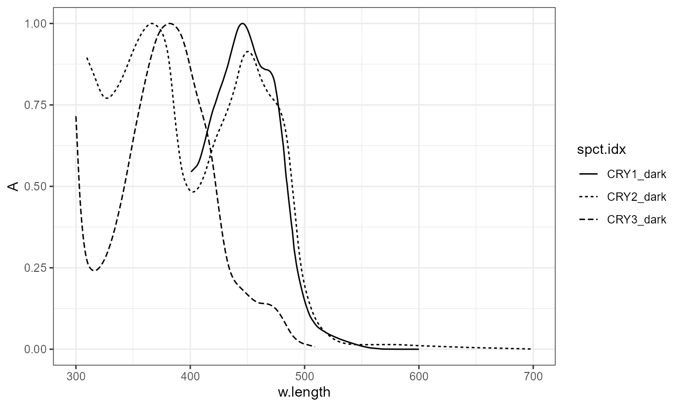

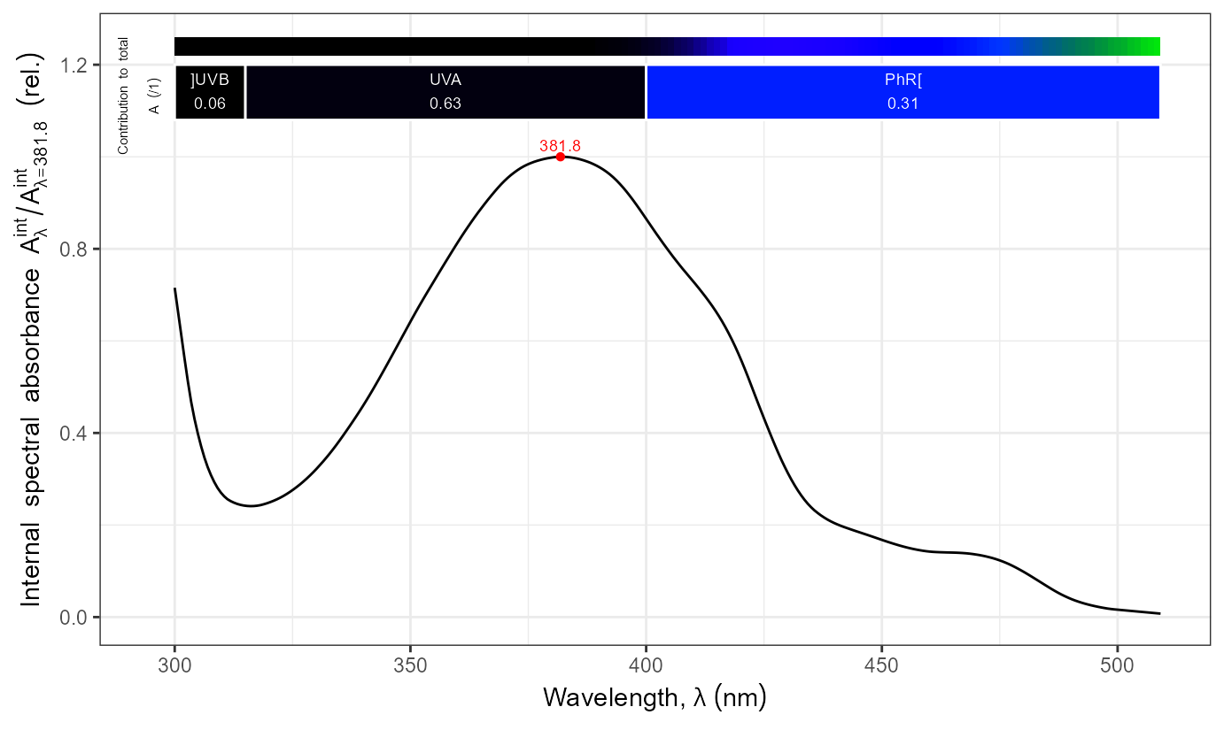
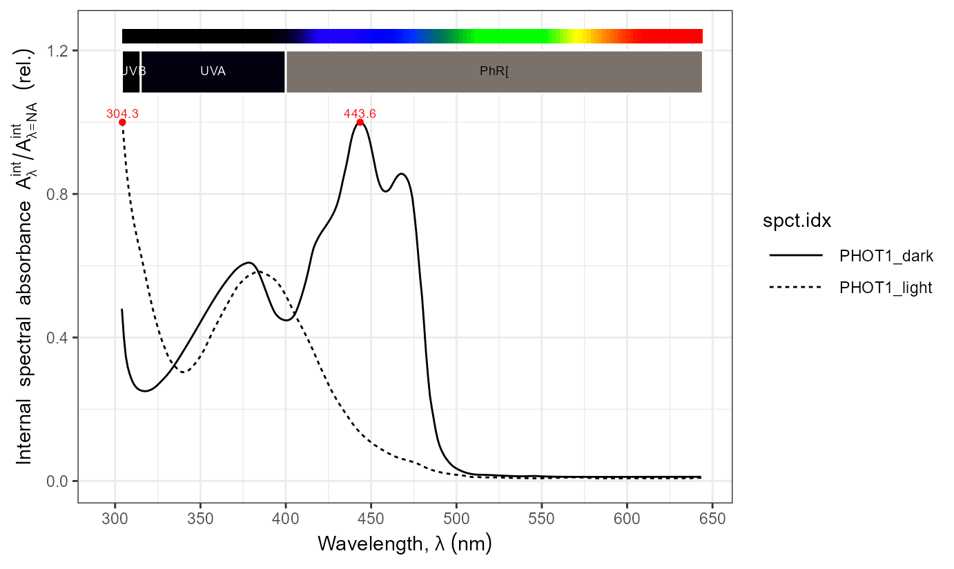
Phototropins: spectral absorbance

names(PHOTs.mspct)

## [1] "PHOT1_fluo"  "PHOT2_fluo"  "PHOT1_dark"  "PHOT1_light"

autoplot(PHOTs.mspct[c("PHOT1_fluo", "PHOT2_fluo")]) +
  expand_limits(x = 300)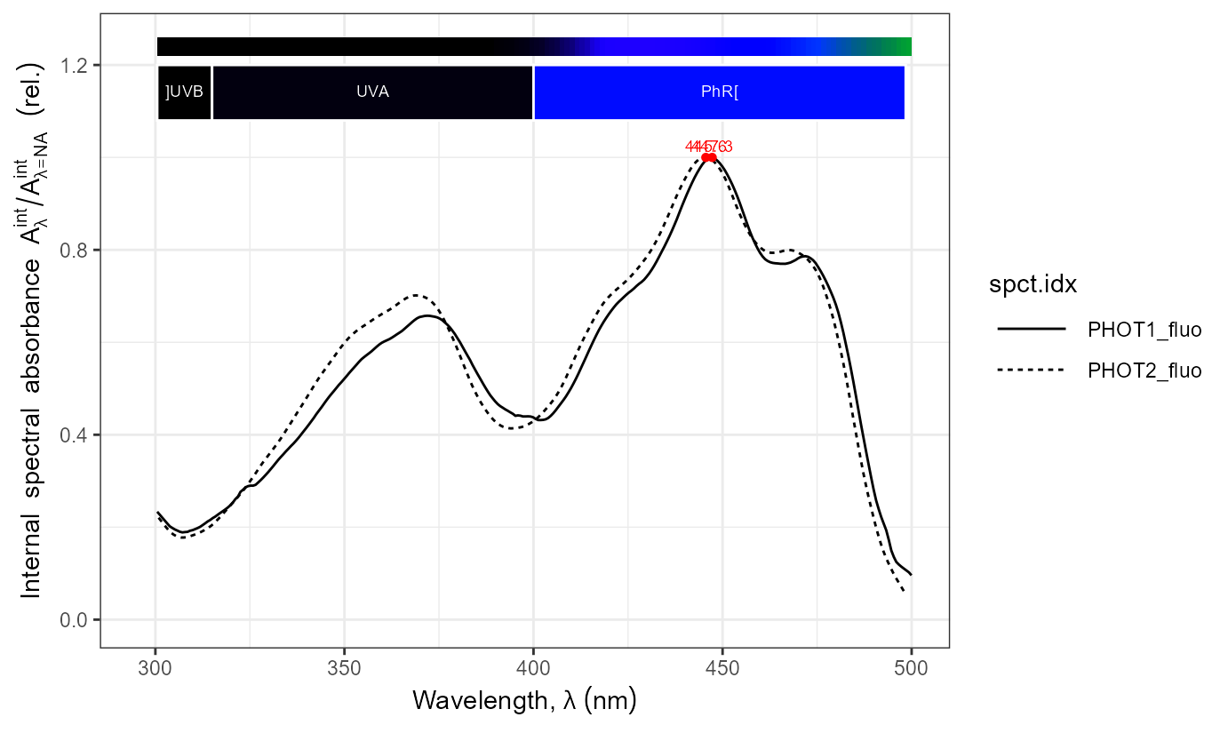

autoplot(PHOTs.mspct[c("PHOT1_dark", "PHOT1_light")])

UVR8: spectral absorbance

autoplot(UVR8s.mspct)

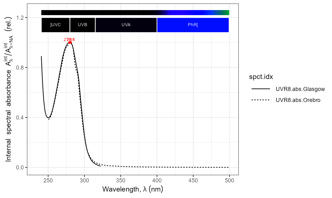
Zeitloupe proteins: spectral absorbance

names(ZTLs.mspct)

## [1] "ZTL_dark"  "ZTL_light"

autoplot(ZTLs.mspct) +
  expand_limits(x = 300)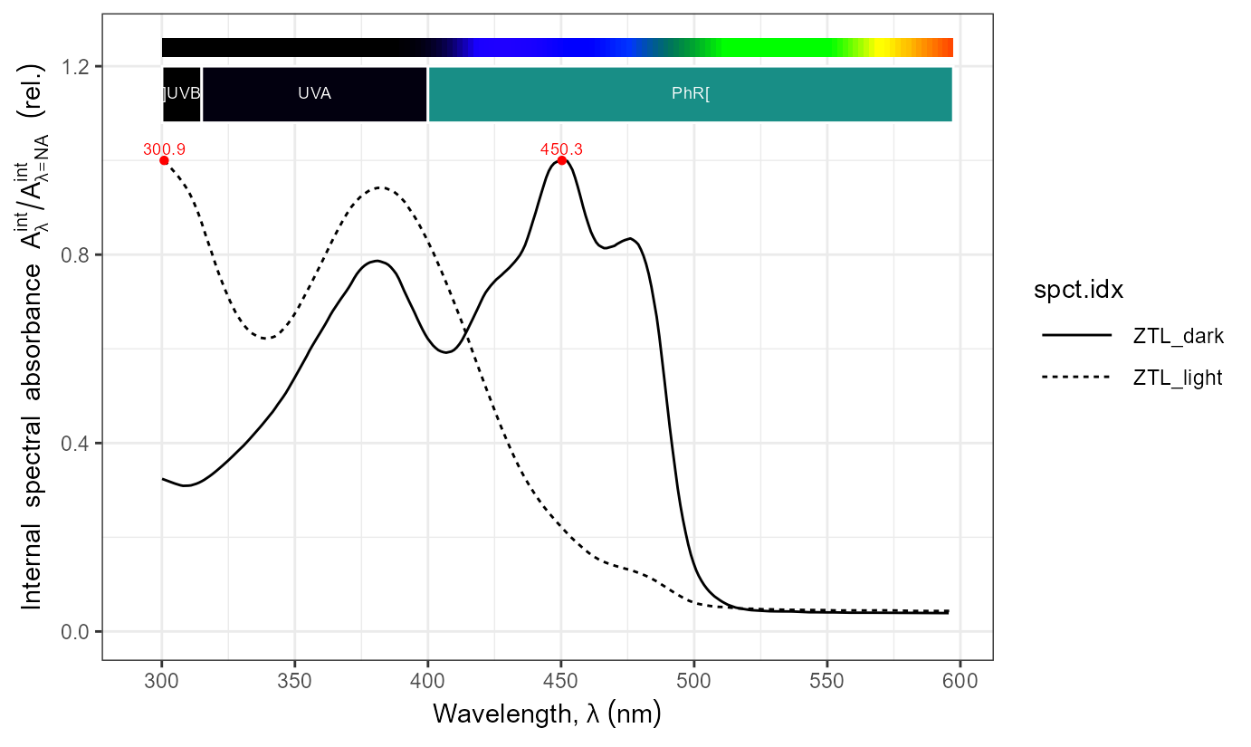

Mass pigments

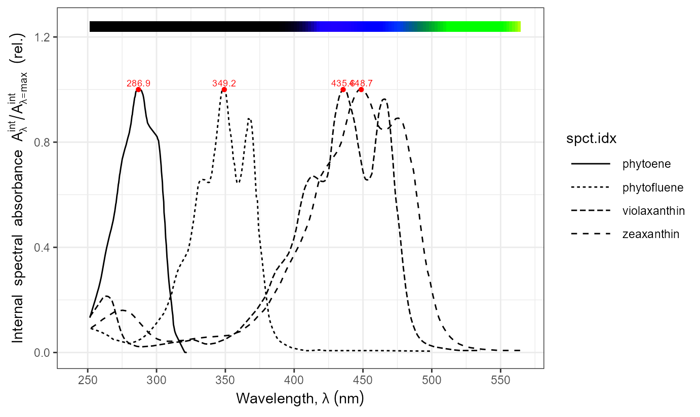
Carotenoids

A_as_default()

names(carotenoids.mspct)

## [1] "beta_carotene"    "dihydro_lycopene" "lycopene"         "lutein"          
## [5] "phytoene"         "phytofluene"      "violaxanthin"     "zeaxanthin"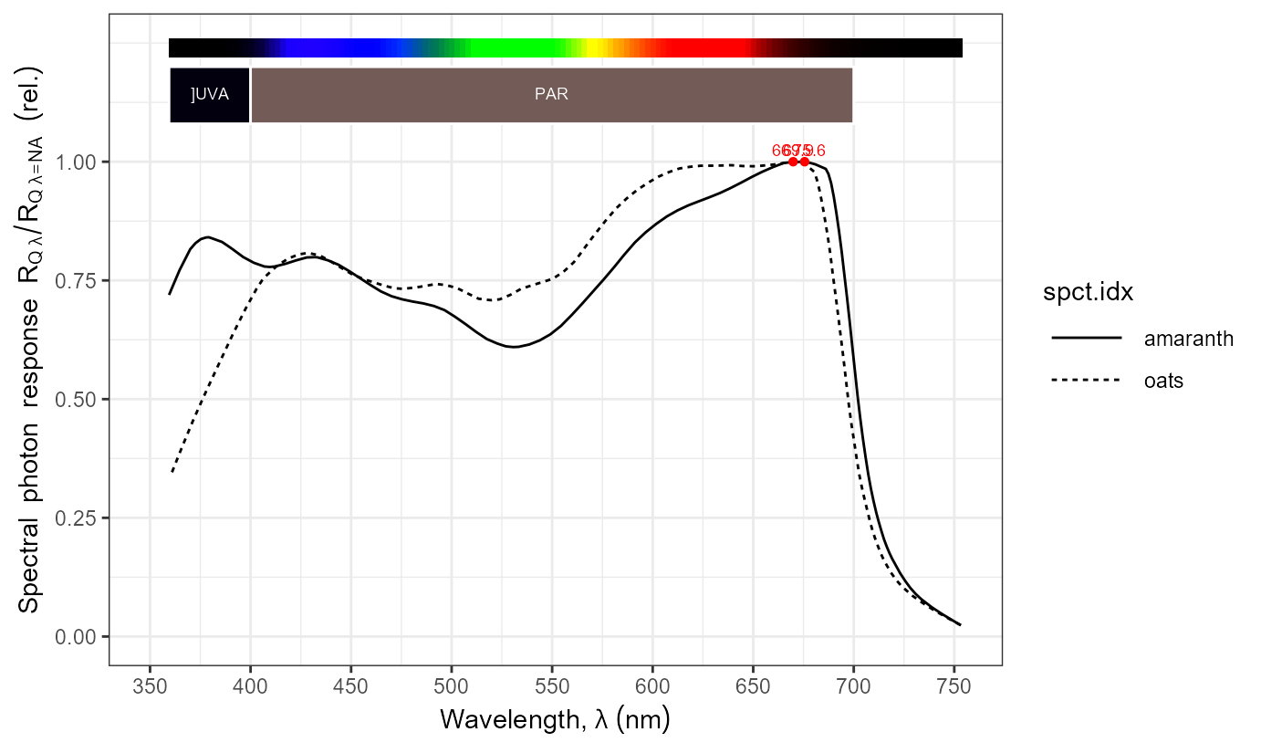

autoplot(carotenoids.mspct[1:4], 
         annotations = c("-", "labels", "boxes"))

autoplot(carotenoids.mspct[5:length(carotenoids.mspct)], 
         annotations = c("-", "labels", "boxes"))

Chlorophylls

A_as_default()

names(chlorophylls.mspct)

## [1] "Chl_a_MethOH" "Chl_a_DME"    "Chl_b_DME"

autoplot(chlorophylls.mspct[c("Chl_a_DME", "Chl_b_DME")])

autoplot(chlorophylls.mspct[c("Chl_a_DME", "Chl_a_MethOH")])

Fluorescence

names(chlorophylls_fluorescence.mspct)

## [1] "Chl_a_MethOH" "Chl_a_DME"    "Chl_b_DME"

autoplot(chlorophylls_fluorescence.mspct[c("Chl_a_DME", "Chl_b_DME")])

autoplot(chlorophylls_fluorescence.mspct[c("Chl_a_DME", "Chl_a_MethOH")])

Leaves

Optical properties

Tfr_as_default()

names(Solidago_altissima.mspct)

## [1] "lower_adax" "lower_abax" "upper_adax" "upper_abax"

autoplot(Solidago_altissima.mspct$lower_adax)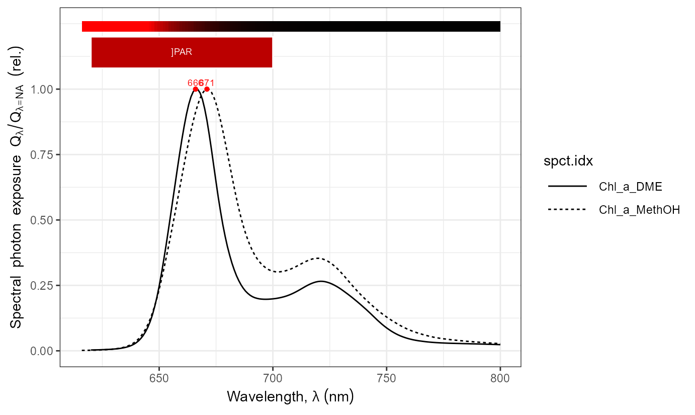

autoplot(Solidago_altissima.mspct$lower_abax)

autoplot(as.filter_mspct(Betula_ermanii.mspct))

autoplot(as.reflector_mspct(Betula_ermanii.mspct))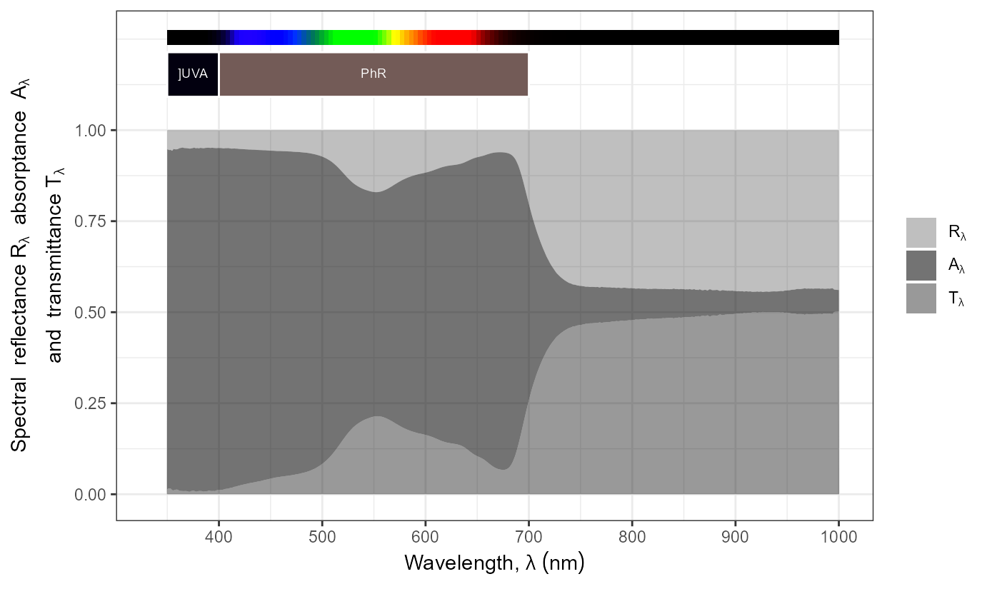

Fluorescence: UV excited

names(leaf_fluorescence.mspct)

## [1] "wheat_Fo_ex355nm"

autoplot(leaf_fluorescence.mspct$wheat_Fo_ex355nm)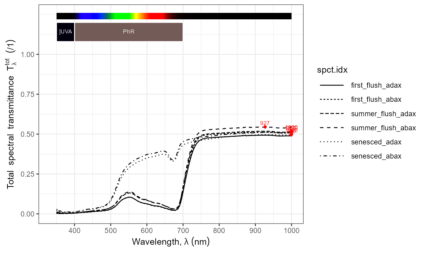

Photosynthesis: action spectra

photon_as_default()

names(McCree_photosynthesis.mspct)

## [1] "amaranth" "oats"     "lettuce"

autoplot(McCree_photosynthesis.mspct)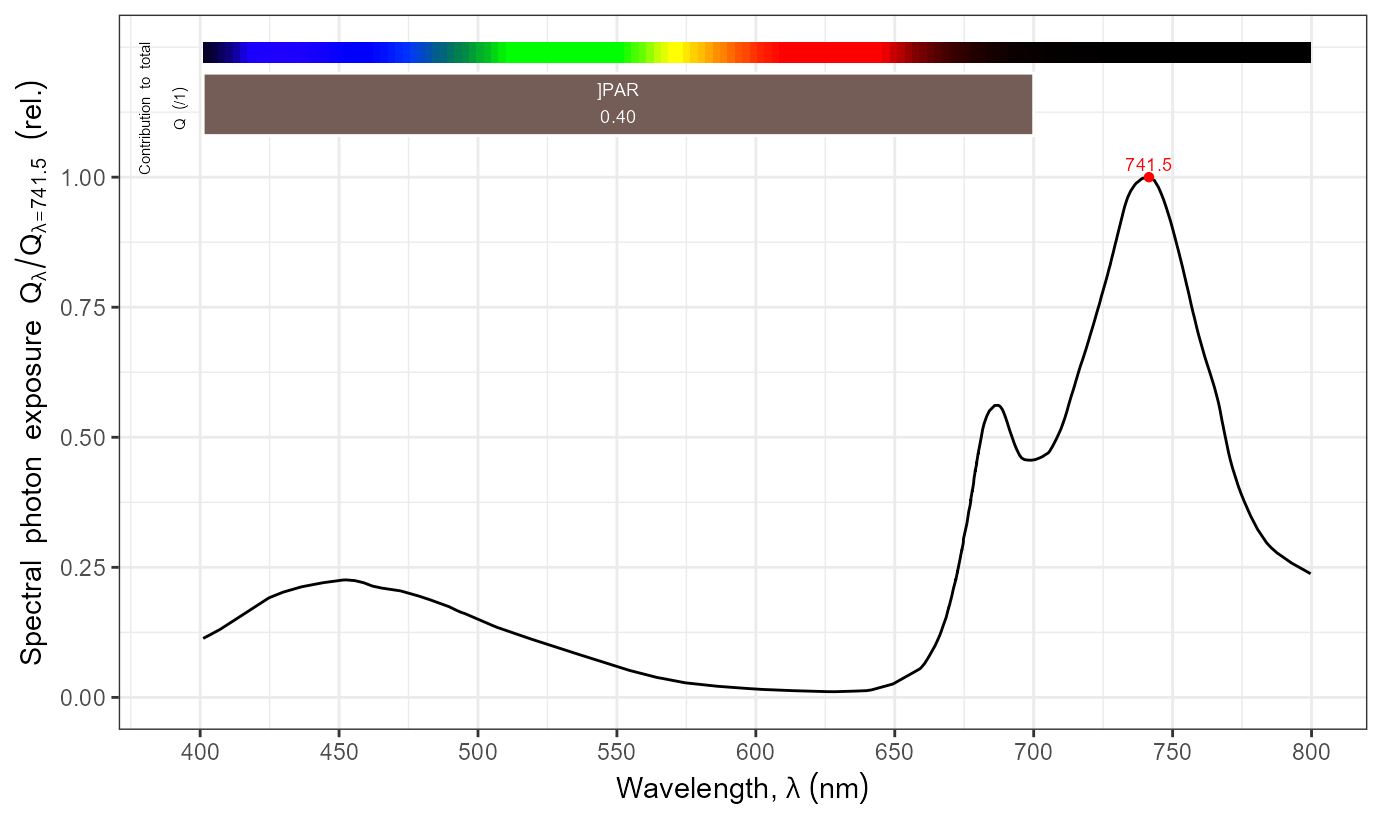

Stomatal conductance

The functions described in this section are available in ‘photobiologyPlants’ (>= 0.6.2).

While in meteorology it is common to use stomatal resistances expressed based of volume, in plant sciences their expression as molar conductances is the norm. The conversion depends on the molar volume of air, which here is treated as an ideal gas. The molar volume is a function of temperature and pressure.

1 / gs_mol2vol(0.150) # mol m-2 s-1 -> s m-2

## [1] 276.1464

# mol m-2 s-1 -> s m-2
1 / gs_mol2vol(0.150, temperature = 5, pressure = 98e3)

## [1] 282.5177

Stomatal conductance is directly dependent on the diffusion coefficient (D) which depends on the chemical species, temperature and pressure.

gs_c_from_gs_w(0.150) # mol m-2 s-1

## [1] 0.09109934

Estimation of stomatal conductance from the measured size of the stomatal pore is challenging, both because of the difficulty in doing the measurements and because the equation used is based on an approximation to the real shape of stomata.

gs_w <-
  gs_w_from_size(length = 10e-6, # m
                 width = 5e-6, # m
                 depth = 20e-6, # m
                 n = 50e6, # m^-2 (stomatal density)
                 temperature = 30) |>  # C
  gs_vol2mol(temperature = 30, pressure = 101e3) # C, Pa
gs_w # for water vapour mol m-2 s-1

## [1] 0.09914633

gs_w * 1e3 # for water vapour mmol m-2 s-1

## [1] 99.14633

gs_c_from_gs_w(gs_w) * 1e3 # for CO2 mmol m-2 s-1

## [1] 60.21443

These functions rely on computation of the volumetric diffusion coefficients,

D_water(c(0, 10, 20, 30, 40))

## [1] 2.12e-05 2.27e-05 2.42e-05 2.57e-05 2.72e-05

D_CO2(c(0, 10, 20, 30, 40))

## [1] 1.29e-05 1.38e-05 1.47e-05 1.56e-05 1.65e-05

and the molar volume of an ideal gas.

molar_vol(c(0, 10, 20, 30, 40))

## [1] 0.02241825 0.02323898 0.02405971 0.02488045 0.02570118

molar_vol(temperature = 25, pressure = c(98e3, 100e3, 102e3))

## [1] 0.02529407 0.02478819 0.02430215

Vegetation

The functions described in this section have been migrated from package ‘photobiology’ (>= 0.12.0) to ‘photobiologyPlants’ (>= 0.6.0).

Reference evapotranspiration

Evapotranspiration is the combined water fluxes between a vegetation canopy and the atmosphere, It is the sum of transpiration (water that evaporates inside leaves and flows through stomata) and evaporation (water that evaporated from the soil and other surfaces, including from the wet outer surfaces of plants and their leaves). Measured evapotranspiration is described as actual evapotranspiration (\mathrm{ET}), the maximum rate of evapotranspiration of short vegetation canopy is called reference evapotranspiration (\mathrm{ET}_\mathrm{ref}), also described as potential evapotranspiration (\mathrm{PET})). Potential evapotranspiration can be measured on irrigated vegetation, but can also be estimated from meteorological conditions. Supported methods are the current FAO recommended and some earlier ones still in use.

Instantaneous \mathrm{ET}_\mathrm{ref} expressed in mm\ h^{-1} can be obtained with ET_ref().

ET_ref(temperature = 20, # C
       water.vp = water_RH2vp(relative.humidity = 70, # RH%
                              temperature = 20), # C -> Pa
       wind.speed = 0, # m s-1
       net.irradiance = 100) # W m-2

## [1] 0.172792

Daily \mathrm{ET}_\mathrm{ref} expressed in mm\ d^{-1} can be obtained with ET_ref_day()

ET_ref_day(temperature = 20, # C daily mean
           water.vp = 1636.616, # Pa daily mean
           wind.speed = 5, # m s-1 daily mean
           net.radiation = 15e6) # 15 MJ / d / m2 daily total !

## [1] 7.199597

As many of other factions in the package, these functions are vectorized.

ET_ref(temperature = 20, # C
       water.vp = water_RH2vp(relative.humidity = (1:9) * 10, # RH%
                              temperature = 20), # C -> Pa
       wind.speed = 5, # m s-1
       net.irradiance = 10) # W m-2

## [1] 0.01733964 0.01733277 0.01732590 0.01731904 0.01731217 0.01730530 0.01729843
## [8] 0.01729157 0.01728470

Potential evapotranspiration is in most situation proportional to the available radiant energy.

ET_ref_irrad.df <-
  data.frame(irrad = (1:40) * 10,
             ET.ref = ET_ref(temperature = 20, # C
                             water.vp = water_RH2vp(relative.humidity = 70, # RH%
                                                    temperature = 20), # C -> Pa
                             wind.speed = 5, # m s-1
                             net.irradiance = (1:40) * 10) # W m-2
  )
ggplot(ET_ref_irrad.df, aes(irrad, ET.ref)) +
  geom_line() +
  labs(x = expression("Global radiation "*(W~m^{-2})),
       y = expression("Reference evapotranspiration "*(mm~h^{-1})))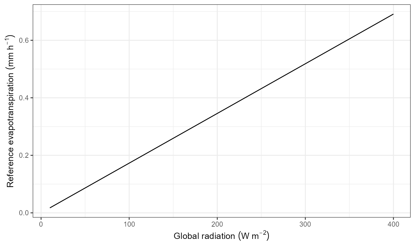

Function net_irradiance() simplifies the computation of net irradiance, needed as input for the computation of reference evapotranspiration.

Water vapour in air

Water vapour partial pressure in air depends on temperature and on whether air is in equilibrium with liquid water or ice.Not considered here, solutes in water and surface interactions also affect the equilibrium. The examples below use the default equation for the computation of saturated water vapour pressure. The default is Tetens’ equation from 1930. Currently supported methods are "tetens", modified "magnus", "wexler" and "goff.gratch".

water_vp_sat(20) # temperature in C, partial pressure in Pa

## [1] 2338.023

water_vp_sat(20) * 1e-3 # temperature in C, partial pressure in kPa

## [1] 2.338023

vp_sat.df <- data.frame(temperature = -20:100,
                        vp.sat = c(water_vp_sat(-20:-1, over.ice = TRUE),
                                   water_vp_sat(0:100)) * 1e-3)

ggplot(vp_sat.df, aes(temperature, vp.sat)) +
  geom_line() +
  labs(x = "Temperature (C)", y = "Water valour pressure at saturation (kPa)")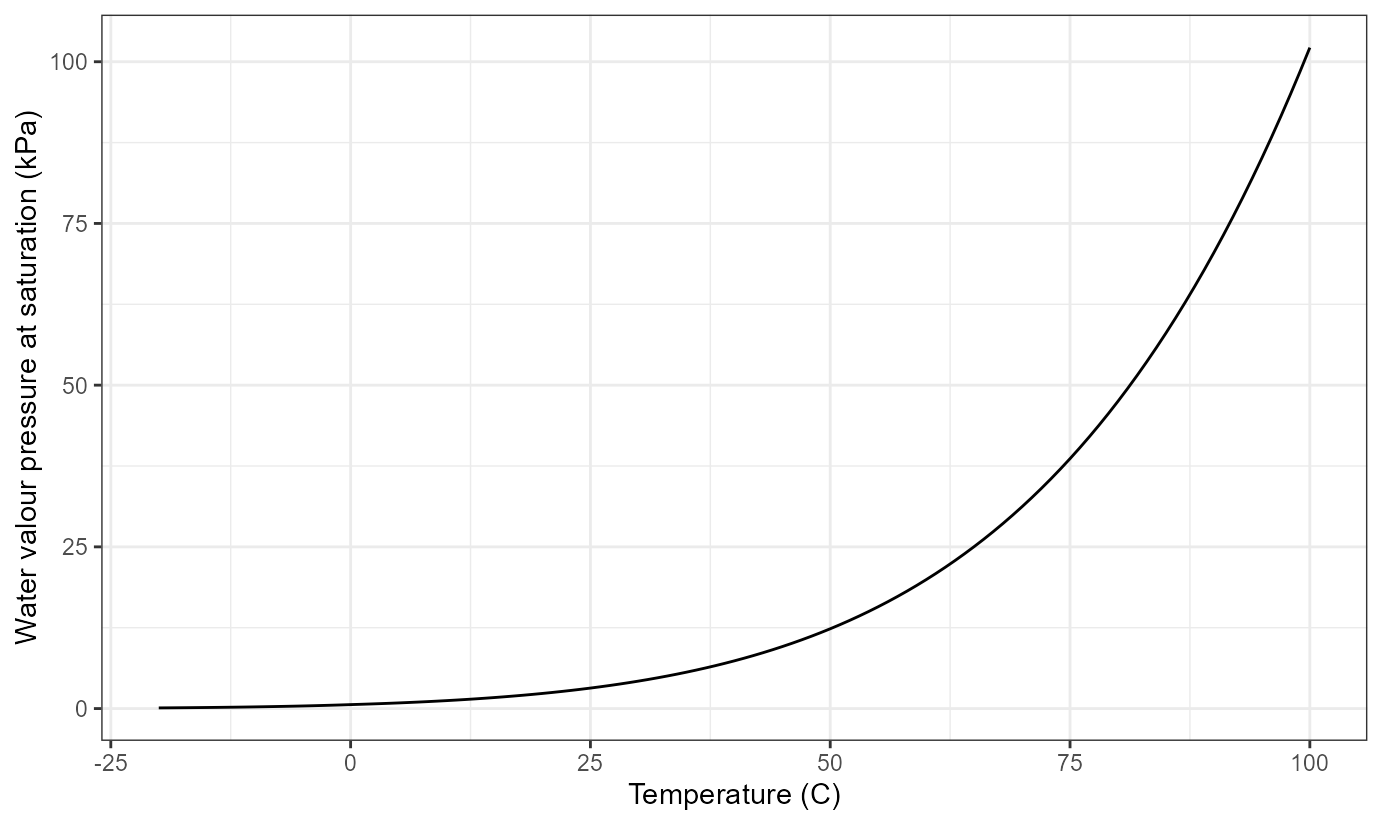

Conversion of water vapour pressure to relative humidity and vice versa is based on the curve shown in the figure above.

water_vp2RH(1000, 25) # Pa and C -> RH%

## [1] 31.57191

water_vp2mvc(1000, 25) # Pa and C ->  mass per volume g m-3

## [1] 7.264556

The reverse conversion functions are water_RH2vp(), water_mvc2vp().

If we know the actual vapour pressure we can compute at which temperature this pressure would the saturating (RH = 100%), or dew point.

water_dp(1000) # Pa -> C

## [1] 6.973856

If the vapour pressure is very low, instead of dew point we have to compute the freezing point.

water_fp(500) # Pa -> C

## [1] -2.40697

Function water_vp_sat_slope() can be used to compute the slope of the curve in the figure above as a function of air temperature, and function psychrometric_constant() to compute the psychrometric constant as a function of air temperature.

Package ‘photobiologyPlants’ 0.6.1.1.9000

Pedro J. Aphalo

2025-11-14