Equation, p-value, R^2 of major axis regression

stat_ma_eq fits model II regressions. From the fitted model it generates several labels including the equation, p-value, coefficient of determination (R^2), and number of observations.

Usage

stat_ma_eq(
  mapping = NULL,
  data = NULL,
  geom = "text_npc",
  position = "identity",
  ...,
  formula = NULL,
  method = "lmodel2:MA",
  method.args = list(),
  n.min = 2L,
  range.y = NULL,
  range.x = NULL,
  nperm = 99,
  eq.with.lhs = TRUE,
  eq.x.rhs = NULL,
  small.r = FALSE,
  small.p = FALSE,
  coef.digits = 3,
  coef.keep.zeros = TRUE,
  rr.digits = 2,
  theta.digits = 2,
  p.digits = max(1, ceiling(log10(nperm))),
  label.x = "left",
  label.y = "top",
  hstep = 0,
  vstep = NULL,
  output.type = NULL,
  na.rm = FALSE,
  orientation = NA,
  parse = NULL,
  show.legend = FALSE,
  inherit.aes = TRUE
)

Arguments

mapping: The aesthetic mapping, usually constructed with aes. Only needs to be set at the layer level if you are overriding the plot defaults.
data: A layer specific dataset, only needed if you want to override the plot defaults.
geom: The geometric object to use display the data
position: The position adjustment to use for overlapping points on this layer
...: other arguments passed on to layer. This can include aesthetics whose values you want to set, not map. See layer for more details.
formula: a formula object. Using aesthetic names x and y instead of original variable names.
method: function or character If character, "MA", "SMA" , "RMA" or "OLS", alternatively "lmodel2" or the name of a model fit function are accepted, possibly followed by the fit function's method argument separated by a colon (e.g. "lmodel2:MA"). If a function different to lmodel2(), it must accept arguments named formula, data, range.y, range.x and nperm and return a model fit object of class lmodel2.
method.args: named list with additional arguments.
n.min: integer Minimum number of distinct values in the explanatory variable (on the rhs of formula) for fitting to the attempted.
range.y, range.x: character Pass "relative" or "interval" if method "RMA" is to be computed.
nperm: integer Number of permutation used to estimate significance.
eq.with.lhs: If character the string is pasted to the front of the equation label before parsing or a logical (see note).
eq.x.rhs: character this string will be used as replacement for "x" in the model equation when generating the label before parsing it.
small.r, small.p: logical Flags to switch use of lower case r and p for coefficient of determination and p-value.
coef.digits: integer Number of significant digits to use for the fitted coefficients.
coef.keep.zeros: logical Keep or drop trailing zeros when formatting the fitted coefficients and F-value.
rr.digits, theta.digits, p.digits: integer Number of digits after the decimal point to use for R^2, theta and P-value in labels. If Inf, use exponential notation with three decimal places.
label.x, label.y: numeric with range 0..1 "normalized parent coordinates" (npc units) or character if using geom_text_npc() or geom_label_npc(). If using geom_text() or geom_label() numeric in native data units. If too short they will be recycled.
hstep, vstep: numeric in npc units, the horizontal and vertical step used between labels for different groups.
output.type: character One of "expression", "LaTeX", "text", "markdown" or "numeric".
na.rm: a logical indicating whether NA values should be stripped before the computation proceeds.
orientation: character Either "x" or "y" controlling the default for formula.
parse: logical Passed to the geom. If TRUE, the labels will be parsed into expressions and displayed as described in ?plotmath. Default is TRUE if output.type = "expression" and FALSE otherwise.
show.legend: logical. Should this layer be included in the legends? NA, the default, includes if any aesthetics are mapped. FALSE never includes, and TRUE always includes.
inherit.aes: If FALSE, overrides the default aesthetics, rather than combining with them. This is most useful for helper functions that define both data and aesthetics and shouldn't inherit behaviour from the default plot specification, e.g. borders.

Value

A data frame, with a single row and columns as described under

Computed variables. In cases when the number of observations is less than n.min a data frame with no rows or columns is returned rendered as an empty/invisible plot layer.

Details

This stat can be used to automatically annotate a plot with \(R^2\), \(P\)-value, \(n\) and/or the fitted model equation. It supports linear major axis (MA), standard major axis (SMA) and ranged major axis (RMA) regression by means of function lmodel2. Please see the documentation, including the vignette of package 'lmodel2' for details. The parameters in stat_ma_eq() follow the same naming as in function lmodel2().

It is important to keep in mind that although the fitted line does not depend on whether the \(x\) or \(y\) appears on the rhs of the model formula, the numeric estimates for the parameters do depend on this.

A ggplot statistic receives as data a data frame that is not the one passed as argument by the user, but instead a data frame with the variables mapped to aesthetics. stat_ma_eq() mimics how stat_smooth() works, except that only linear regression can be fitted. Similarly to these statistics the model fits respect grouping, so the scales used for x and y should both be continuous scales rather than discrete.

The minimum number of observations with distinct values can be set through parameter n.min. The default n.min = 2L is the smallest possible value. However, model fits with very few observations are of little interest and using a larger number for n.min than the default is usually wise.

Note

For backward compatibility a logical is accepted as argument for eq.with.lhs. If TRUE, the default is used, either "x" or "y", depending on the argument passed to formula. However, "x" or "y" can be substituted by providing a suitable replacement character string through eq.x.rhs. Parameter orientation is redundant as it only affects the default for formula but is included for consistency with ggplot2::stat_smooth().

Methods in lmodel2 are all computed always except for RMA that requires a numeric argument to at least one of range.y or range.x. The results for specific methods are extracted a posteriori from the model fit object. When a function is passed as argument to method, the method can be passed in a list to method.args as member method. More easily, the name of the function can be passed as a character string together with the lmodel2-supported method.

R option OutDec is obeyed based on its value at the time the plot is rendered, i.e., displayed or printed. Set options(OutDec = ",") for languages like Spanish or French.

Aesthetics

stat_ma_eq understands x and y, to be referenced in the formula while the weight aesthetic is ignored. Both x and y must be mapped to numeric variables. In addition, the aesthetics understood by the geom ("text" is the default) are understood and grouping respected.

Transformation of x or y within the model formula is not supported by stat_ma_eq(). In this case, transformations should never be applied in the model formula, but instead in the mapping of the variables within aes.

Computed variables

If output.type different from "numeric" the returned tibble contains columns listed below. If the fitted model does not contain a given value, the label is set to character(0L).

x,npcx: x position
y,npcy: y position
eq.label: equation for the fitted polynomial as a character string to be parsed
rr.label: \(R^2\) of the fitted model as a character string to be parsed
p.value.label: P-value if available, depends on method.
theta.label: Angle in degrees between the two OLS lines for lines estimated from y ~ x and x ~ y linear model (lm) fits.
n.label: Number of observations used in the fit.
grp.label: Set according to mapping in aes.
method.label: Set according method used.
r.squared, theta, p.value, n: numeric values, from the model fit object

If output.type is "numeric" the returned tibble contains columns listed below. If the model fit function used does not return a value, the variable is set to NA_real_.

x,npcx: x position
y,npcy: y position
coef.ls: list containing the "coefficients" matrix from the summary of the fit object
r.squared, theta, p.value, n: numeric values, from the model fit object
grp.label: Set according to mapping in aes.
b_0.constant: TRUE is polynomial is forced through the origin
b_i: One or two columns with the coefficient estimates

To explore the computed values returned for a given input we suggest the use of geom_debug as shown in the last examples below.

Examples

# generate artificial data
set.seed(98723)
my.data <- data.frame(x = rnorm(100) + (0:99) / 10 - 5,
                      y = rnorm(100) + (0:99) / 10 - 5,
                      group = c("A", "B"))

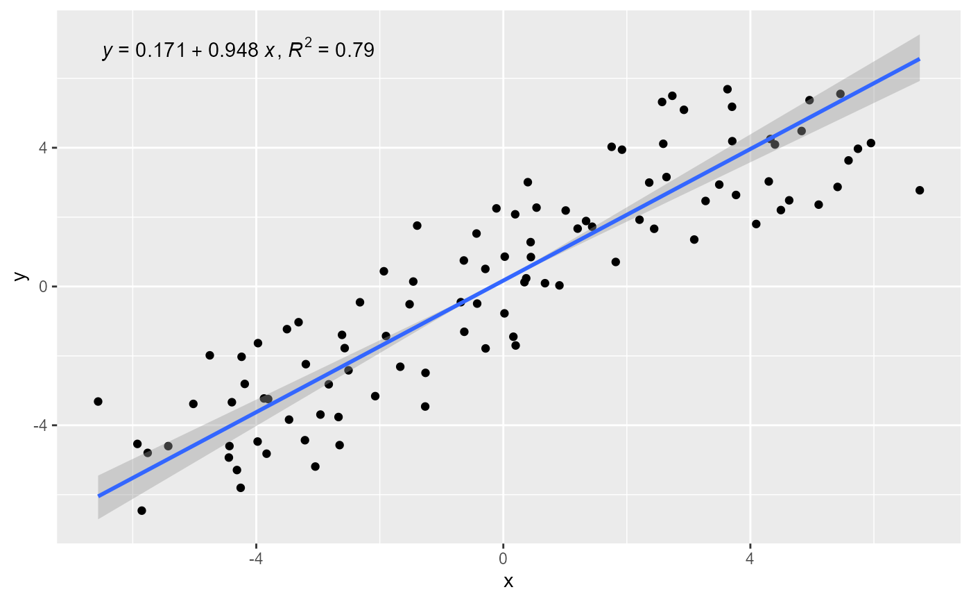
# using defaults (major axis regression)
ggplot(my.data, aes(x, y)) +
  geom_point() +
  stat_ma_line() +
  stat_ma_eq()


# use_label() can assemble and map a combined label
ggplot(my.data, aes(x, y)) +
  geom_point() +
  stat_ma_line(method = "MA") +
  stat_ma_eq(use_label(c("eq", "R2", "P")))


ggplot(my.data, aes(x, y)) +
  geom_point() +
  stat_ma_line(method = "MA") +
  stat_ma_eq(use_label(c("R2", "P", "theta", "method")))


# using ranged major axis regression
ggplot(my.data, aes(x, y)) +
  geom_point() +
  stat_ma_line(method = "RMA",
               range.y = "interval",
               range.x = "interval") +
  stat_ma_eq(use_label(c("eq", "R2", "P")),
             method = "RMA",
             range.y = "interval",
             range.x = "interval")


# No permutation-based test
ggplot(my.data, aes(x, y)) +
  geom_point() +
  stat_ma_line(method = "MA") +
  stat_ma_eq(use_label(c("eq", "R2")),
             method = "MA",
             nperm = 0)
#> No permutation test will be performed
#> Warning: 'p.digits < 2' Likely information loss!


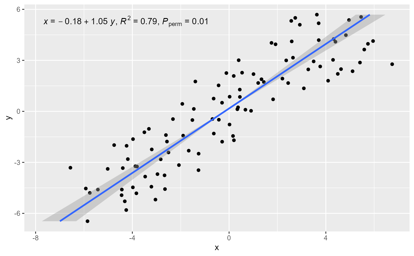
# explicit formula "x explained by y"
ggplot(my.data, aes(x, y)) +
  geom_point() +
  stat_ma_line(formula = x ~ y) +
  stat_ma_eq(formula = x ~ y,
             use_label(c("eq", "R2", "P")))


# modifying both variables within aes()
ggplot(my.data, aes(log(x + 10), log(y + 10))) +
  geom_point() +
  stat_poly_line() +
  stat_poly_eq(use_label("eq"),
               eq.x.rhs = "~~log(x+10)",
               eq.with.lhs = "log(y+10)~~`=`~~")


# grouping
ggplot(my.data, aes(x, y, color = group)) +
  geom_point() +
  stat_ma_line() +
  stat_ma_eq()


# labelling equations
ggplot(my.data,
       aes(x, y,  shape = group, linetype = group, grp.label = group)) +
  geom_point() +
  stat_ma_line(color = "black") +
  stat_ma_eq(use_label(c("grp", "eq", "R2"))) +
  theme_classic()


# Inspecting the returned data using geom_debug()
# This provides a quick way of finding out the names of the variables that
# are available for mapping to aesthetics with after_stat().

gginnards.installed <- requireNamespace("gginnards", quietly = TRUE)

if (gginnards.installed)
  library(gginnards)

# default is output.type = "expression"
if (gginnards.installed)
  ggplot(my.data, aes(x, y)) +
    geom_point() +
    stat_ma_eq(geom = "debug")

#> [1] "Summary of input 'data' to 'draw_panel()':"
#>   npcx npcy                  label                               eq.label
#> 1   NA   NA italic(R)^2~`=`~"0.79" italic(y)~`=`~0.171 + 0.948*~italic(x)
#>                 rr.label              p.value.label              theta.label
#> 1 italic(R)^2~`=`~"0.79" italic(P)[perm]~`=`~"0.01" italic(theta)~`=`~"6.67"
#>               n.label grp.label         method.label r.squared    theta p.value
#> 1 italic(n)~`=`~"100"        -1 "method: lmodel2:MA" 0.7917998 6.665222    0.01
#>     n  fm.method fm.class fm.formula fm.formula.chr        x        y PANEL
#> 1 100 lmodel2:MA  lmodel2      y ~ x          y ~ x -6.56061 5.687505     1
#>   group
#> 1    -1

if (FALSE) {
if (gginnards.installed)
  ggplot(my.data, aes(x, y)) +
    geom_point() +
    stat_ma_eq(aes(label = after_stat(eq.label)),
               geom = "debug",
               output.type = "markdown")

if (gginnards.installed)
  ggplot(my.data, aes(x, y)) +
    geom_point() +
    stat_ma_eq(geom = "debug", output.type = "text")

if (gginnards.installed)
  ggplot(my.data, aes(x, y)) +
    geom_point() +
    stat_ma_eq(geom = "debug", output.type = "numeric")
}