Cloudflecks: big data example

Introduction

At the moment this vignette has the double purpose of keeping track of my progress and testing the performance of the functions in the package. My aim is to analyse a large set of high frequency time series measurements of sunlight at seven different wavebands done with broadband sensors over one summer.

The data set will be large with seven variables and a few hundred millions of time points. During daytime measurements were acquired in bursts of 18000 time points in 15 min every 30 min.

The effect of clouds is intermittent and varies in intensity gradually. Using quantiles, mean, MAD and variance on the irradiance, and on the running differences is one possible approach. However, a recent additional approach is based on detecting change points in the running differences as a basis to quantify the duration and amplitude of cloud/shade flecks.

The data are in large text files saved with the software PC400 from Campbell Scientific, the supplier of the data logger used to collect the data set.

The first step is to read-in the data and split it into “chunks” of data from 18000 consecutive observations at the gaps between the “bursts” of observations, discarding any incomplete sets and any data measured at a lower frequency. At this stage running differences for time stamps need to be computed, and running differences for the measured variables can also be added at the same time.

The smaller values in the running differences are most likely the result of measurement “noise” and could be “cleaned” before the next steps. The differences can be used directly or discretized based on their sign.

Current state

The reading of the data from the 3.7GB text file into a tibble is the slowest step. Other computations are fast even with the functions are coded fully in R.

Set up

library(dplyr)
#> 
#> Attaching package: 'dplyr'
#> The following objects are masked from 'package:stats':
#> 
#>     filter, lag
#> The following objects are masked from 'package:base':
#> 
#>     intersect, setdiff, setequal, union
library(photobiologyInOut)
#> Loading required package: photobiology
#> Loading required package: SunCalcMeeus
#> Documentation at https://docs.r4photobiology.info/
library(photobiologyFlecks)
library(ggplot2)

Read raw data

Read data from a CSV file as saved by Campbell Scientific’s PC400 program containing data acquired with a CR6 data logger. These data are not calibrated!

# file.name <- "data-raw/Viikki Tower_TableMilliSecond.dat"
file.name <- "F:\\aphalo\\research-data\\data-weather\\weather-viikki-field-2025\\data-logged\\data-2025-08-25\\TOA5_1449.TableMilliSecond.dat"
file.size(file.name)
#> [1] 3667693021
file.mtime(file.name)
#> [1] "2025-08-25 17:42:02 EEST"

# limit number of chunks read
chunk_nrows <- 18000
# nchunks <- 50
# temp_file.name <- "H:/data-temp/some-chunks-tb.rda"

nchunks <- Inf
temp_file.name <- "H:/data-temp/all-chunks-tb.rda"

All rows from a large file will be used in the examples. Reading and decoding the text file is slow, so we create a temporary binary file and use it if it exists or create it after reading the text file if not. Reading from the temp file a 3.7GB tibble takes only about 10 s of both elapsed and user time while reading the DAT file takes nearly 450 s of elapsed time and 3600 s of user time on a computer with a processor with 6 physical cores (12 logical ones). The numbers do not add, so user time must be based on logical cores (12) with multi-threading. Anyway, 240 s of system time, give 3820 of user + system time, indicating an average use of nearly 9 cores during 7 min 24 s.

system.time(
  if (!file.exists(temp_file.name)) {
    all_chunks.tb <- 
      read_csi_dat(file.name, n_max = chunk_nrows * nchunks) |>
      dplyr::select(-RECORD)
    save(all_chunks.tb, file = temp_file.name)
  } else {
    load(temp_file.name)
  }
)
#>    user  system elapsed 
#>    9.94    0.37   10.34

ncol(all_chunks.tb) # all chunks read
#> [1] 9
colnames(all_chunks.tb)
#> [1] "TIMESTAMP"      "PAR_Den_CS"     "UVBf_Den"       "UVAf_Den"      
#> [5] "UVA1f_Den"      "Bluef_Den"      "Greenf_Den"     "Red_Den_Ap"    
#> [9] "Far_red_Den_Ap"
nrow(all_chunks.tb)
#> [1] 34732552

Load calibrated data

CURRENTLY SKIPPED

rm(all_chunks.tb)

Read data from a CSV file as saved by Campbell Scientific’s PC400 program containing data acquired with a CR6 data logger. These data are not calibrated!

# file.name <- "data-raw/Viikki Tower_TableMilliSecond.dat"
file.name <- "F:\\aphalo\\research-data\\data-weather\\weather-viikki-field-2025\\data-logged\\data-2025-08-25\\TOA5_1449.TableMilliSecond.dat"
file.size(file.name)
file.mtime(file.name)

infoRDS(file.name)
all_chunks.tb <- readRDS(file.name)

Split data into chunks

The time series data of sunlight have been measured in 15-min-long bursts separated by 15 min with no data acquisition. Data from each burst will be analysed separately. For this the data frame has to be split at the gaps between bursts.

system.time(
  # keep all qty columns, add differences
  chunks.ls <-
    split_chunks(all_chunks.tb,
                 qty.name = NULL,
                 time.step = 0.051,
                 chunk.min.time = 14 * 60,
                 chunk.min.rows = 1.8e4,
                 verbose = FALSE)
)
#> Found 1925 chunks with length(s) 18000
#>    user  system elapsed 
#>   15.39    5.17   20.61

Some checks

length(chunks.ls) == length(unique(names(chunks.ls)))
#> [1] TRUE
nchunks_found <- length(chunks.ls)

str(chunks.ls[[1]], give.attr = FALSE)
#> tibble [18,000 × 18] (S3: tbl_df/tbl/data.frame)
#>  $ TIMESTAMP          : POSIXct[1:18000], format: "2025-07-01 21:30:00" "2025-07-01 21:30:00" ...
#>  $ PAR_Den_CS         : num [1:18000] 0.351 0.376 0.395 0.386 0.361 ...
#>  $ UVBf_Den           : num [1:18000] 3.29 2.03 2.95 2.63 2.68 ...
#>  $ UVAf_Den           : num [1:18000] 6.72 6.71 6.73 6.72 6.73 ...
#>  $ UVA1f_Den          : num [1:18000] 10.9 10.9 10.9 10.9 10.9 ...
#>  $ Bluef_Den          : num [1:18000] 8.84 8.84 8.83 8.83 8.83 ...
#>  $ Greenf_Den         : num [1:18000] 4.42 4.44 4.42 4.43 4.42 ...
#>  $ Red_Den_Ap         : num [1:18000] 1.63 1.64 1.62 1.64 1.64 ...
#>  $ Far_red_Den_Ap     : num [1:18000] 1.6 1.6 1.61 1.59 1.58 ...
#>  $ TIMESTAMP.diff     : num [1:18000] NA 0.05 0.05 0.05 0.05 ...
#>  $ PAR_Den_CS.diff    : num [1:18000] NA 0.498 0.374 -0.174 -0.498 ...
#>  $ UVBf_Den.diff      : num [1:18000] NA -24.678 17.971 -6.203 0.816 ...
#>  $ UVAf_Den.diff      : num [1:18000] NA -0.201 0.349 -0.192 0.101 ...
#>  $ UVA1f_Den.diff     : num [1:18000] NA 0.1978 0.0927 -0.0857 -0.0216 ...
#>  $ Bluef_Den.diff     : num [1:18000] NA -0.00947 -0.08576 -0.05633 0.07725 ...
#>  $ Greenf_Den.diff    : num [1:18000] NA 0.487 -0.426 0.179 -0.273 ...
#>  $ Red_Den_Ap.diff    : num [1:18000] NA 0.208 -0.4359 0.4557 -0.0173 ...
#>  $ Far_red_Den_Ap.diff: num [1:18000] NA 0.0574 0.1721 -0.3413 -0.2024 ...

Summaries

Statistics

Something seems wrong as I expect a 1 h time shift to be needed!

system.time(
  statistics.tb <- 
    summarize_chunks(chunks.ls, 
                     add.times = TRUE, 
                     tz = "EET",
                     time.shift = 0,
                     add.solar.times = TRUE,
                     geocode = data.frame(lon = 25.019212, lat = 60.226805),
                     verbose = FALSE)
)
#> Summarized 1925 chunks
#>    user  system elapsed 
#>   59.81    9.06   67.00
save(statistics.tb, file = gsub("\\.[rR]da$", ".summaries.rda", temp_file.name))

colnames(statistics.tb)
#>  [1] "PAR_Den_CS"          "UVBf_Den"            "UVAf_Den"           
#>  [4] "UVA1f_Den"           "Bluef_Den"           "Greenf_Den"         
#>  [7] "Red_Den_Ap"          "Far_red_Den_Ap"      "TIMESTAMP.diff"     
#> [10] "PAR_Den_CS.diff"     "UVBf_Den.diff"       "UVAf_Den.diff"      
#> [13] "UVA1f_Den.diff"      "Bluef_Den.diff"      "Greenf_Den.diff"    
#> [16] "Red_Den_Ap.diff"     "Far_red_Den_Ap.diff" "parameter"          
#> [19] "chunk"               "date"                "time"               
#> [22] "solar.time"
length(unique(statistics.tb[["chunk"]])) == nchunks_found
#> [1] TRUE
length(unique(statistics.tb[["time"]])) == nchunks_found
#> [1] TRUE

statistics.tb |>
  select(time, PAR_Den_CS, parameter) |>
ggplot(aes(time, PAR_Den_CS)) +
  geom_point(size = 0.1) +
  facet_wrap(facets = vars(parameter), scales = "free_y")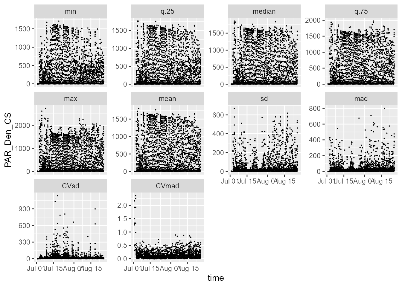

statistics.tb |>
  select(time, date, PAR_Den_CS, parameter) |>
  filter(parameter == "mean") |>
ggplot(aes(as_tod(time), PAR_Den_CS)) +
  geom_point(size = 0.1) +
  facet_wrap(facets = vars(date))

statistics.tb |>
  select(solar.time, date, UVBf_Den, parameter) |>
  filter(parameter == "mean") |>
ggplot(aes(solar.time, UVBf_Den)) +
  geom_point(size = 0.1) +
  facet_wrap(facets = vars(date))

statistics.tb |>
  select(time, date, PAR_Den_CS, parameter) |>
  filter(parameter == "CVsd") |>
ggplot(aes(as_tod(time), PAR_Den_CS)) +
  geom_point(size = 0.1) +
  facet_wrap(facets = vars(date))

statistics.tb |>
  select(solar.time, date, UVBf_Den, parameter) |>
  filter(parameter == "median") |>
ggplot(aes(solar.time, UVBf_Den)) +
  geom_point(size = 0.1) +
  facet_wrap(facets = vars(date))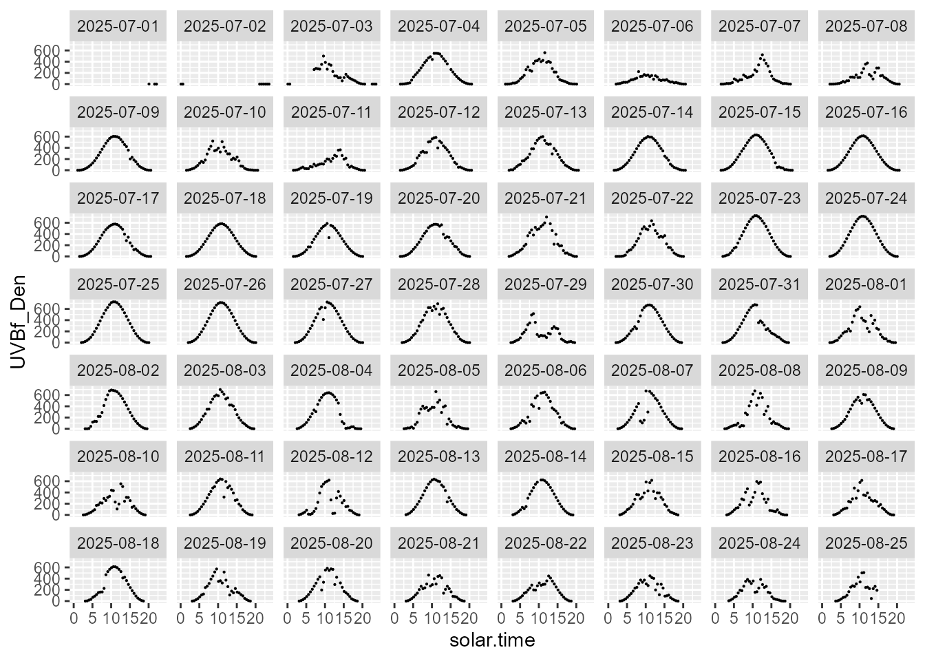

statistics.tb |>
  select(time, date, PAR_Den_CS, parameter) |>
  filter(parameter == "CVmad") |>
ggplot(aes(as_tod(time), PAR_Den_CS)) +
  geom_point(size = 0.1) +
  facet_wrap(facets = vars(date))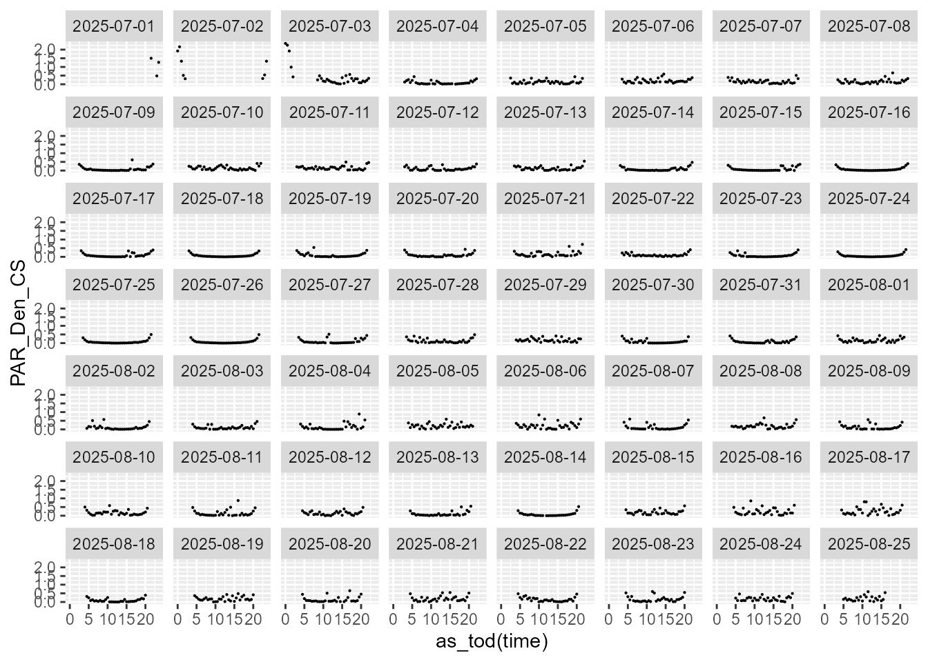

statistics.tb |>
  select(solar.time, date, UVBf_Den, parameter) |>
  filter(parameter == "max") |>
ggplot(aes(solar.time, UVBf_Den)) +
  geom_point(size = 0.1) +
  facet_wrap(facets = vars(date))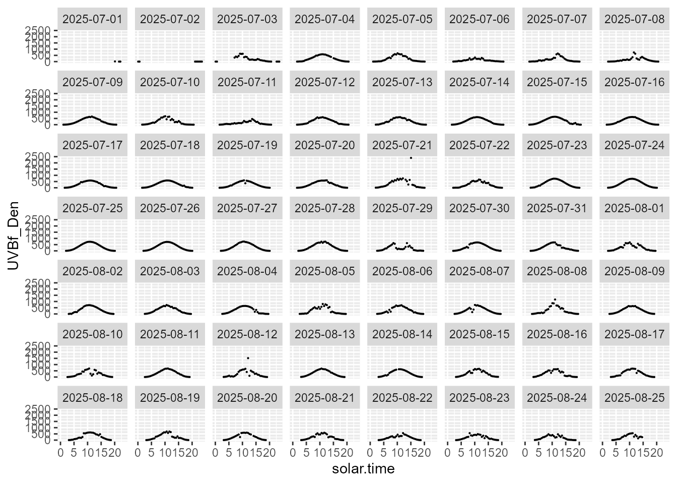

Locating change points

Using `diff()`

Running differences after slight denoising can be used to detect changes in the sign of the local slope, the peaks and valleys of a time series. In other words, the flecks are identified based on local maxima and minima.

We use relative.threshold = 0.20 $\mu mol\,m^{-2}\,s^{-2}$ as the minimum rate of change in irradiance per second to be considered relevant and not discarded as noise.

system.time(
  chunks_dn.ls <- 
    denoise_chunks(chunks.ls, 
                   relative.threshold = 0.20, 
                   add.signs = TRUE)
)
#> Denoised 1925 chunks
#>    user  system elapsed 
#>   12.28    3.86   15.37

In a continuous time series without noise, the derivative is equal to zero at the point where the slope changes sign. In a time series measured at discrete time points, a change in sign must be used as well as a zero value to locate maxima and minima, as the change in slope is most likely to land in-between two time points.

Once de-noised, changes in slope can be detected using sign() to discretize the data into values indicating decrease (-1) , no-change (0) and increase (+1).

Considering the first burst of PAR measurements, we find 597 time steps with change in irradiance.

# time steps with no change
sum(abs(chunks_dn.ls[[1]]$PAR_Den_CS.diff) < 0.20 * 0.05, na.rm = TRUE)
#> [1] 16891
# increasing time steps
sum(chunks_dn.ls[[1]]$PAR_Den_CS.diff > 0.20 * 0.05, na.rm = TRUE)
#> [1] 577
# decreasing time steps
sum(chunks_dn.ls[[1]]$PAR_Den_CS.diff > 0.20 * 0.05, na.rm = TRUE)
#> [1] 577

Subsequently, changes in slope can be located using rle(). In this example all differences are smaller than 5 per thousand of the mean irradiance.

sign_changes.ls <- list()
for (i in names(chunks_dn.ls)) {
  sign_changes.ls[[i]] <- 
    list(rle = rle(chunks_dn.ls[[i]][["PAR_Den_CS.sign"]]))
}
length(sign_changes.ls)
#> [1] 1925

Check that sum of lengths equal length of burst.

sum(sign_changes.ls[[1]][["rle"]][["lengths"]])
#> [1] 18000

sum(sign_changes.ls[[2]][["rle"]][["lengths"]])
#> [1] 18000

Using a reference

Instead of detecting sunflecks as a dynamic temporal process, or local changes in slope, especially in the case of cloud flecks an alternative is to use the estimated clear-sky irradiance as reference and to quantify the size of the deviations, both increases and decreases, in many cases using a fixed threshold. An alternative to using a clear sky simulation is to use a smoothed version of the same data as a reference, a moving median, or a spline-based smoother. However, each of these and the temporal-process approach described above are fundamentally different and describe different properties of the data.

Both observed and reference irradiances need to be available at the same time points. This in some cases can make it necessary to use interpolation to obtain suitable reference data. After this, a simple difference at each time point can be computed and compared against a threshold. As the reference varies in time, the threshold used can be expressed either as an absolute difference or as a relative difference, thus, giving two different quantifications.

Using a quantile smoother

Quantile regression, either of a linear model or a smmothing spline, differs from OLS regression and other common approaches in that it can flexibly be used to find a fitted line that describes a specific quantile. It can be imagined as a combination of a boxplot and a smoother. This approach lets us estimate local deviations from an internal reference different from the local mean or median, say, for example, to identify when irradiance is less than that in the 10% locally highest irradiances.

For vegetation shade a further possibility is to use a quantile regression directly fitted for a target shade threshold.

Package ‘photobiologyFlecks’ 0.0.0.9000

Pedro J. Aphalo

2026-04-22

Introduction

Current state

Set up

Read raw data

Load calibrated data

Split data into chunks

Summaries

Statistics

Locating change points

Using `diff()`

Using a reference

Using a quantile smoother

Cloudflecks: big data example

Package ‘photobiologyFlecks’ 0.0.0.9000

Pedro J. Aphalo

2026-04-22

Introduction

Current state

Set up

Read raw data

Load calibrated data

Split data into chunks

Summaries

Statistics

Locating change points

Using diff()

Using a reference

Using a quantile smoother

Using `diff()`