Geom aesthetics: defaults and targetting
Using packages ‘ggplot2’ (>= 4.0.0) and ‘ggpp’ (>= 0.6.0)
Pedro J. Aphalo
2026-07-02
Source:vignettes/articles/styling-with-themes.Rmd
styling-with-themes.Rmd## Using: 'ggplot2' == 4.0.3 and 'ggpp' == 0.6.1The geom element of ‘ggplot2’ themes
Version 4.0.0 of package ‘ggplot2’ introduced several enhancements to
the use of themes. Of these, the addition of several default aesthetics
of geoms to the theme tree and of
element_geom() are relevant to ‘ggpp’. The code in the
geometries defined in ‘ggpp’ had to be updated to enable support for
themes when used together with ‘ggplot2’ (>= 4.0.0). Examples of
their use are given in this section.
To avoid a hard dependency on ‘ggplot2’ (>= 4.0.0) a fall-back was implemented. The fall back simply provides the same defaults as the default theme from ‘ggplot2’ (< 4.0.0). This fall-back mechanism has been tested with ‘ggplot2’ (== 3.5.2).
One aim of this article is to test what already works and what does not yet work in the version of ‘ggpp’ used to render this article. This article was rendered on 2026-07-02 with ‘ggpp’ version 0.6.1 and ‘ggplot2’ version 4.0.3.
In ‘ggplot2’ (>= 4.0.0) it is possible to change the defaults used by geoms in coordination with the styling of the plot as a whole.
We will use p as a base plot for testing the different
geometries. Because of this, we add mappings to the aesthetics required
by all the different geometries that we will test.
p0 <-
  ggplot(mtcars, aes(x = wt, y = mpg)) +
  geom_point()
Using the default theme.
p0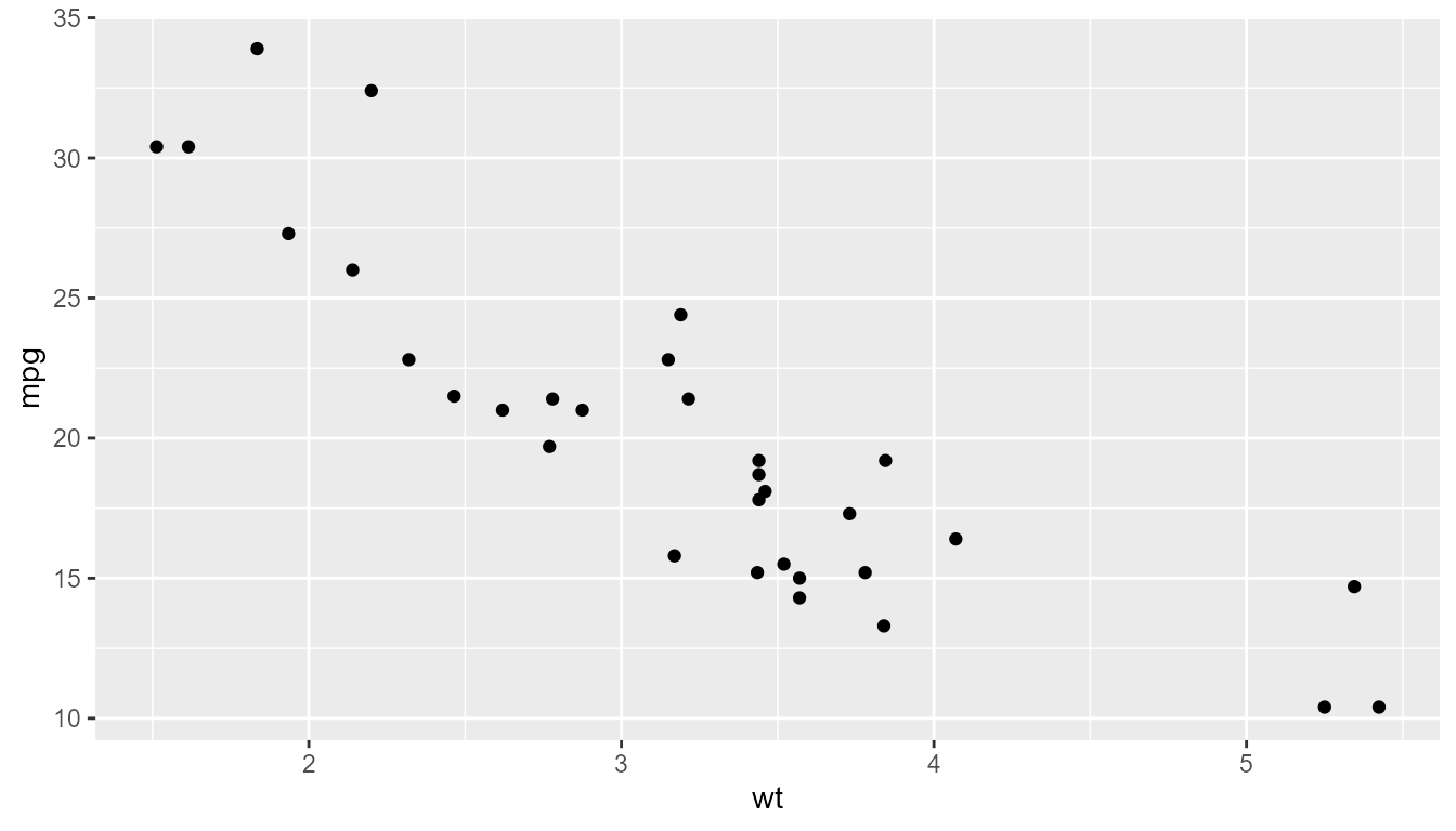
In a call to theme() it is now easy to modify the
default for colour and other aesthetics when used as part
of the overall graphic design. Taking into account that using
set_theme() to set a theme as default we can set the style
of all subsequent plots, this new feature is very convenient.
p0 + theme(geom = element_geom(ink = "blue", paper = "wheat"))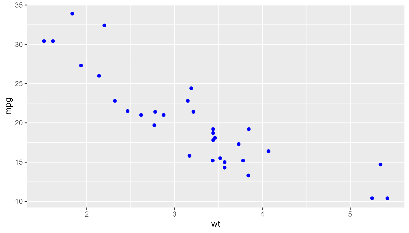
The geom slot of themes was introduced in ‘ggplot2’ (==
4.0.0). As seen above, the entry for geom can be modified
as other slots by calling element_geom() instead of
element_text(), element_rect(), etc.
The defaults from ‘ggplot2’ version 4.0.3 are:
calc_element("geom", get_theme())## <ggplot2::element_geom>
## @ ink : chr "black"
## @ paper : chr "white"
## @ accent : chr "#3366FF"
## @ linewidth : num 0.5
## @ borderwidth: num 0.5
## @ linetype : int 1
## @ bordertype : int 1
## @ family : chr ""
## @ fontsize : num 3.87
## @ pointsize : num 1.5
## @ pointshape : num 19
## @ colour : NULL
## @ fill : NULLWe can see that the defaults for colour and fill are set to
NULL. Unless set explicitly, colour takes its
default value value from ink. While we have only one
aesthetic called linetype used for both lines and column
and label borders, for the plot as a whole, they can be set
differently.
To test if the geometries from ‘ggpp’ obey defaults set through these
theme settings, we modify them in theme_minimal() and set
this as the default theme. Using very unsightly but contrasting colour
we can check more easily if the geometries obey the theme settings.
set_theme(theme_minimal() +
            theme(
              geom = element_geom(
                ink = "darkgreen",
                paper = "wheat",
                accent = "darkred",
                family = "serif",
                linewidth = 0.3,
                linetype = "dotted",
                borderwidth = 1,
                bordertype = "dotted",
                pointsize = 1,
                pointshape = "circle open"
              )
            )
)
We can use the same code as above to retrieve the currently active theme. As expected, it reflects the changes we introduced above.
calc_element("geom", get_theme())## <ggplot2::element_geom>
## @ ink : chr "darkgreen"
## @ paper : chr "wheat"
## @ accent : chr "darkred"
## @ linewidth : num 0.3
## @ borderwidth: num 1
## @ linetype : chr "dotted"
## @ bordertype : chr "dotted"
## @ family : chr "serif"
## @ fontsize : num 3.87
## @ pointsize : num 1
## @ pointshape : chr "circle open"
## @ colour : NULL
## @ fill : NULL
p0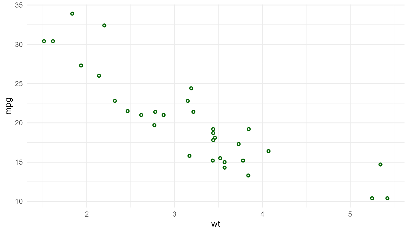
It is also possible to modify them for a specific geom, here,
geom_point().
update_theme(geom.point = element_geom(colour = "blue"))
p0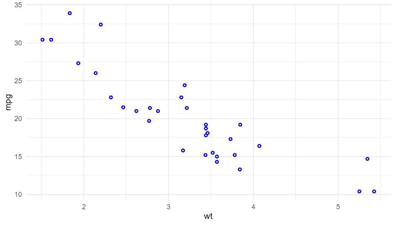
We will use p as a base plot for testing the different
geometries. Because of this, we add mappings to the aesthetics required
by all the different geometries that we will test.
# systematically extract one out of each four rows
my.cars <- mtcars[c(TRUE, FALSE, FALSE, FALSE), ]
my.cars$name <- rownames(my.cars)

p1 <-
  ggplot(my.cars,
         aes(x = wt, y = mpg, label = name,
             xintercept = wt, yintercept = mpg,
             npcx = (wt - min(wt)) / diff(range(wt)),
             npcy = (mpg - (min(mpg))) / diff(range(mpg)))) +
  geom_point()

p <- p1 + expand_limits(x = 6.5)
p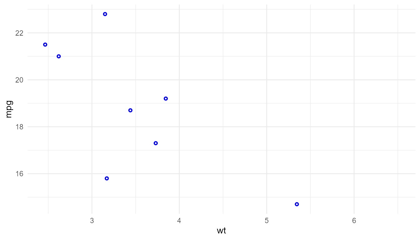
Variations on geom_text()
The expectation is that the text in all these plots look consistent with either green or blue text depending on the specific settings. The positions relative to the points is expected to differ when using roughly calculated NPC.
p + geom_text(hjust = 0, nudge_x = 0.1)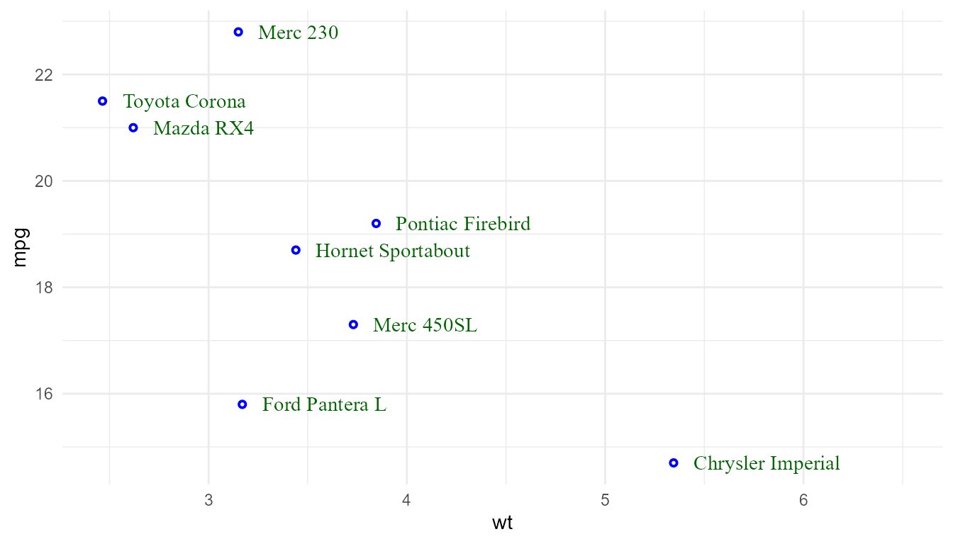
update_theme(geom.text = element_geom(colour = "blue"))
p + geom_text(hjust = 0, nudge_x = 0.1)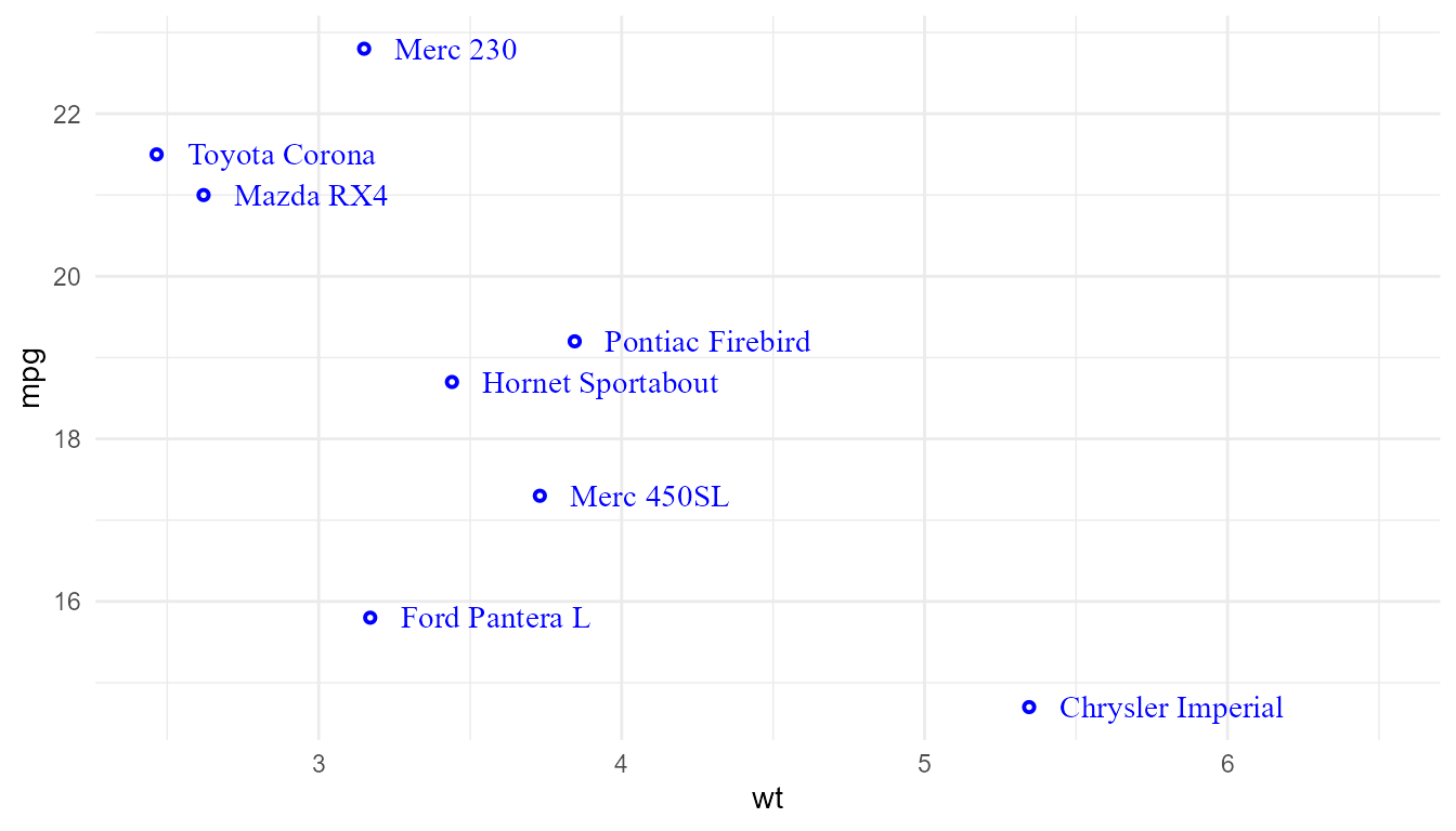
p + geom_text_s(hjust = 0, nudge_x = 0.1)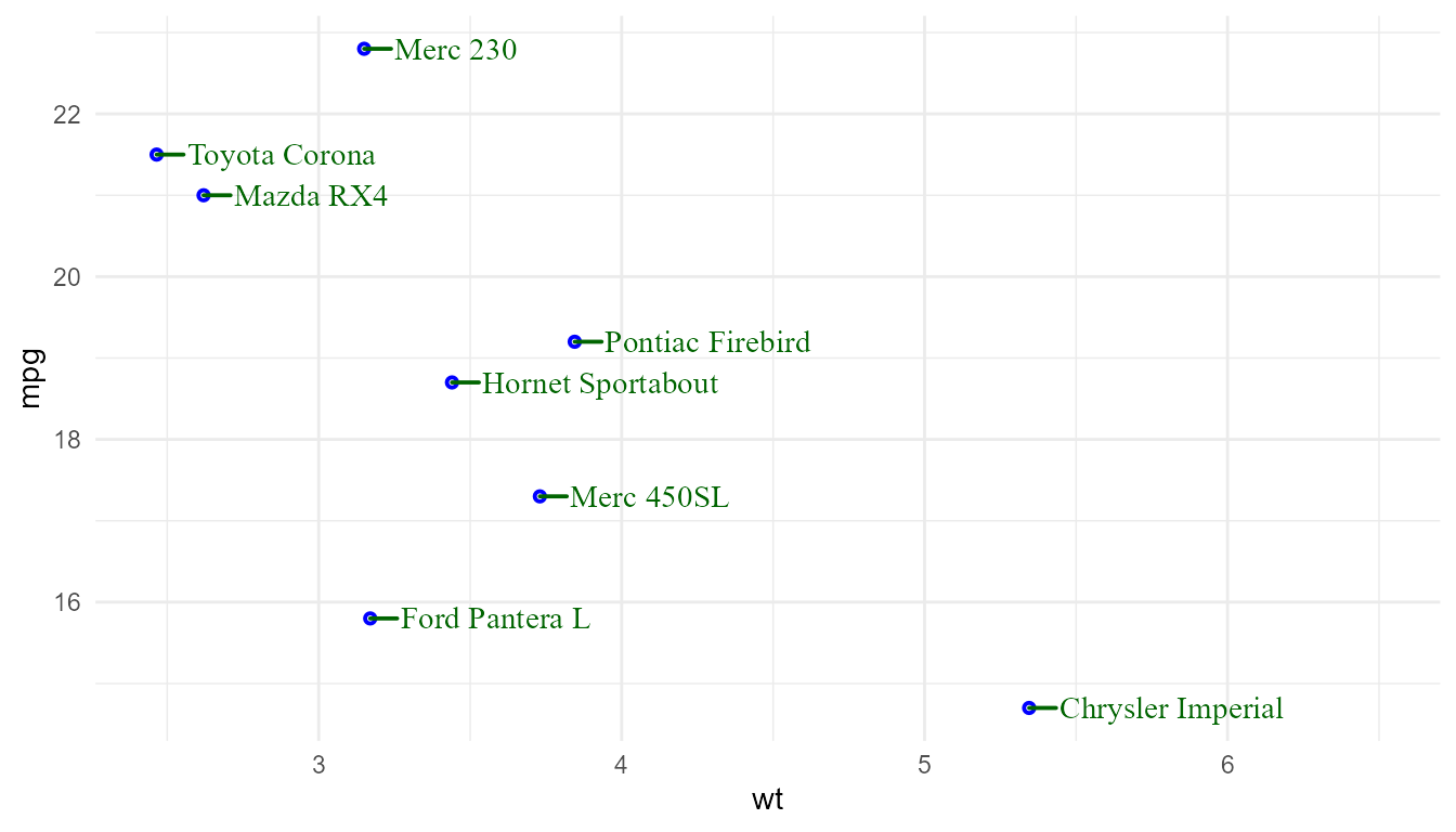
update_theme(geom.text.s = element_geom(colour = "blue"))
p + geom_text_s(hjust = 0, nudge_x = 0.1)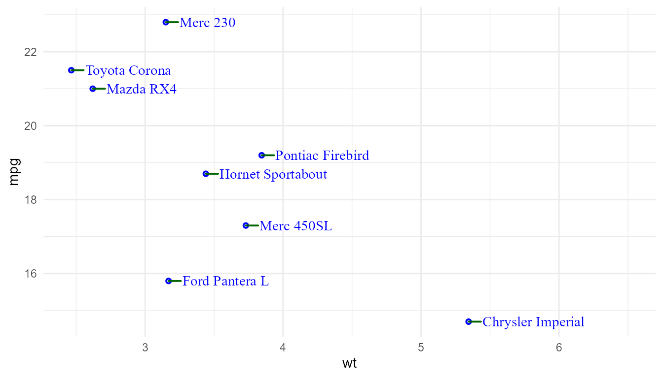
Variations on geom_label()
The expectation is that the labels in all these plots look consistent with either green or blue text on a yellow or transparent background depending on the specific settings. The positions relative to the points is expected to differ when using roughly calculated NPC.
p + geom_label(hjust = 0, nudge_x = 0.1)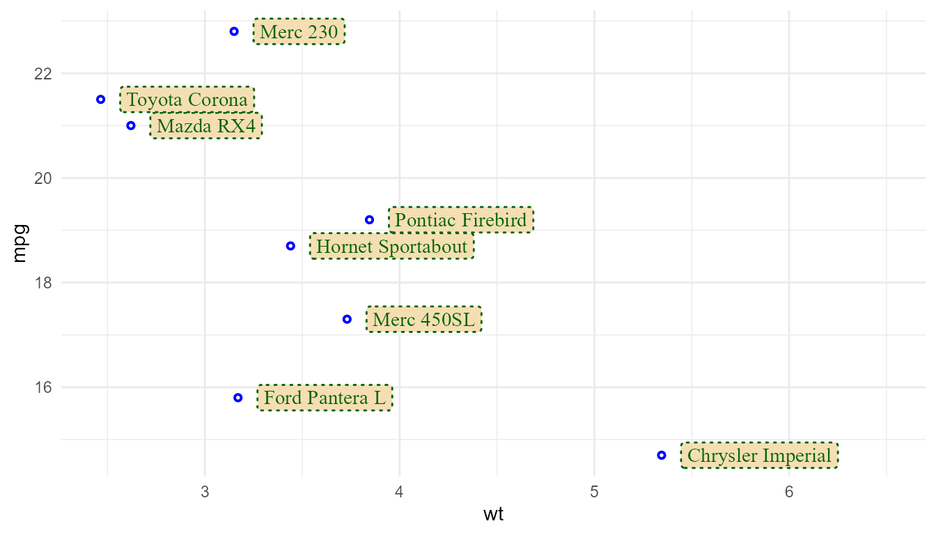
update_theme(geom.label = element_geom(colour = "blue", fill = NA))
p + geom_label(hjust = 0, nudge_x = 0.1)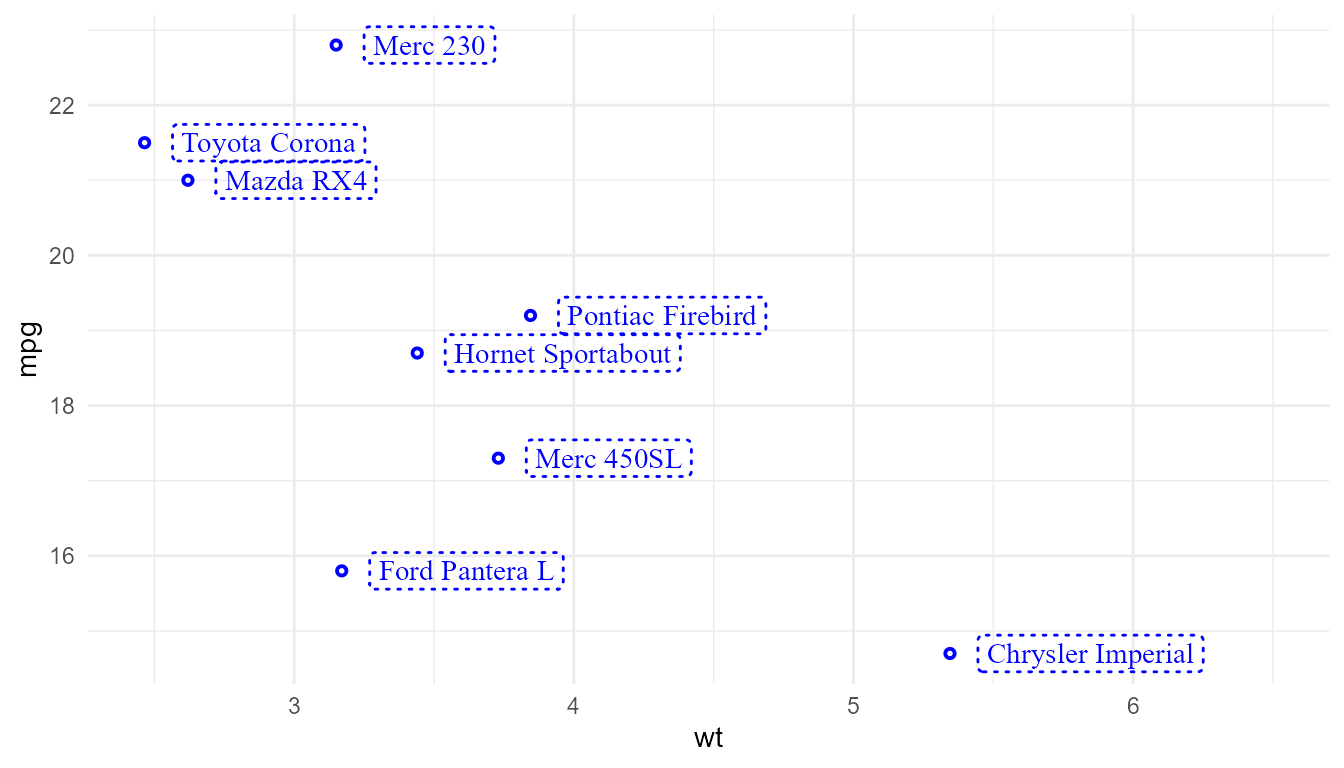
p + geom_label_s(hjust = 0, nudge_x = 0.1)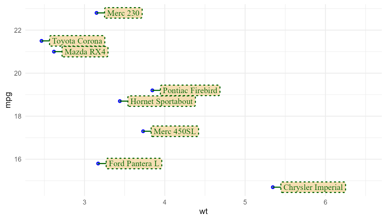
update_theme(geom.label.s = element_geom(colour = "blue", fill = NA))
p + geom_label_s(hjust = 0, nudge_x = 0.1)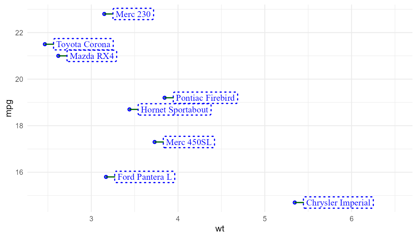
Marks on plot margins
p1 + geom_rug()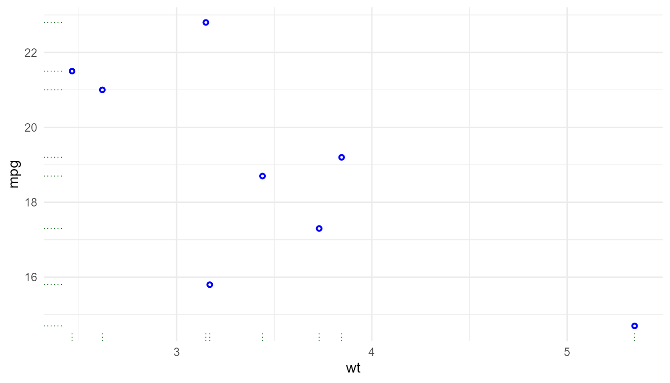
p1 +
  geom_x_margin_point(inherit.aes = TRUE) +
  geom_y_margin_point(inherit.aes = TRUE)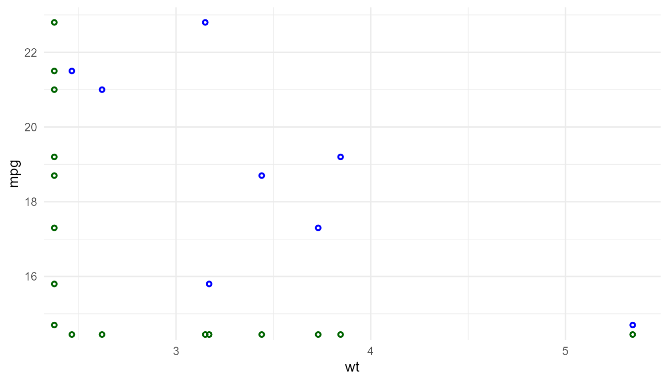
update_theme(geom.x.margin.point = element_geom(colour = "red",
                                                pointshape = 19),
             geom.y.margin.point = element_geom(colour = "orange",
                                                pointshape = "triangle"))
p1 +
  geom_x_margin_point(inherit.aes = TRUE) +
  geom_y_margin_point(inherit.aes = TRUE)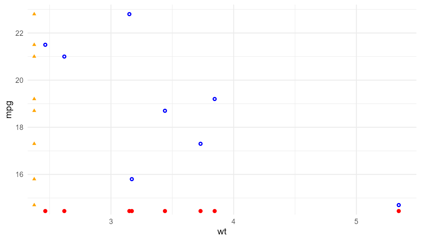
p1 +
  geom_x_margin_arrow(inherit.aes = TRUE) +
  geom_y_margin_arrow(inherit.aes = TRUE)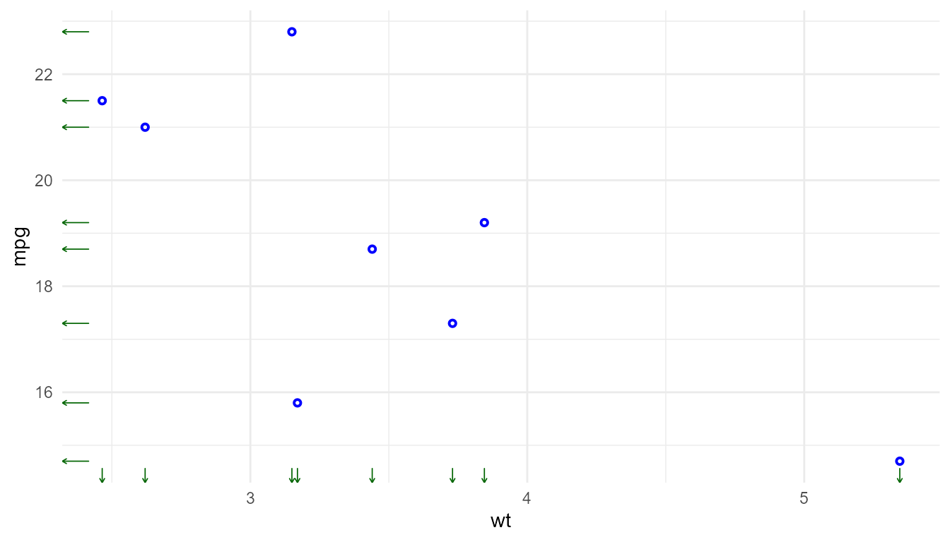
update_theme(geom.x.margin.arrow = element_geom(colour = "green",
                                                pointshape = 19),
             geom.y.margin.arrow = element_geom(colour = "orange",
                                                pointshape = "triangle"))
p1 +
  geom_x_margin_arrow(inherit.aes = TRUE) +
  geom_y_margin_arrow(inherit.aes = TRUE)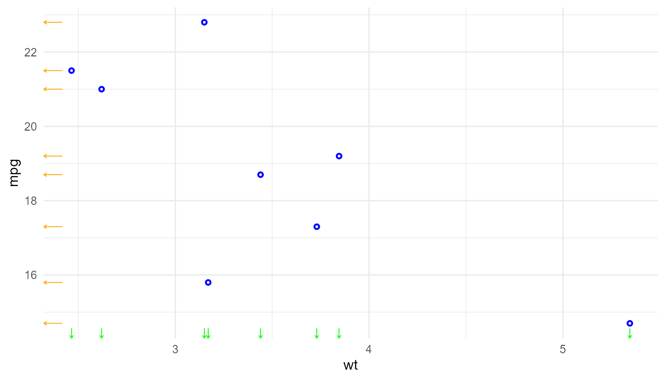
Plot insets
p1 + annotate(geom = "plot", label = p, x = 6, y = 22) Theme defaults for the inset plots are coded into
 p and not
modified when added as an inset. The main and inset plots should both
have blue points.
update_theme(geom.plot = element_geom(colour = "red"))

p1 + annotate(geom = "plot", label = p, x = 6, y = 22)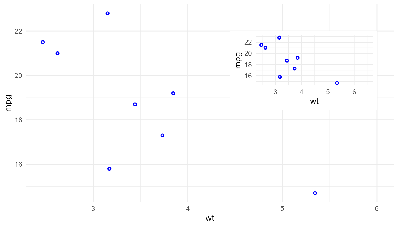
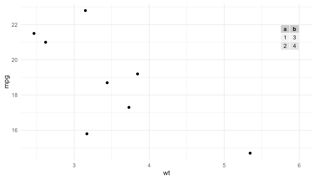
p1 + annotate(geom = "table",
             label = data.frame(a = 1:2, b = 3:4),
             x = 6, y = 22)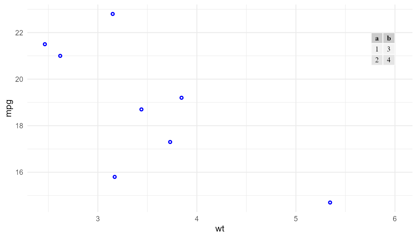
Currently, fontsize and family set in the
plot theme (theme) override those in the table theme
(ttheme) as defaults. The default colour and fill for the
table are always from the table theme. All these defaults, as expected,
can be overridden by mapping a variable or a constant to the respective
aesthetics.
update_theme(geom.table = element_geom(fontsize = 15, family = "sans"))
p1 + annotate(geom = "table",
             label = data.frame(a = 1:2, b = 3:4),
             x = 6, y = 22)
Targetting of mapped aesthetics
Some geometries create simple graphical elements on the layer, and, thus, there is a single possible approach to apply aesthetics to them. For example, the colour of points or lines. Other geometries create graphical elements composed of multiple parts, such labels with text on a background enclosed by a border line. In these more complex graphical elements there are multiple ways in which an aesthetic like colour or transparency can be applied.
In this case two contrasting approaches are possible: 1) defining
multiple aesthetics so that the same conceptual aesthetic (e.g.,
colour) can be independently mapped to different variables
for different components of the graphical object, or 2) adding one
parameter or more parameters to the geometry constructor that indicate
to which graphical element(s) the aesthetic should be applied.
I consider that the targeting of the aesthetic mapping to different elements of a graphical object is related to graphical design and not part of the data representation. Thus ‘ggpp’ follows the second approach. The idea is that a single colour mapping assigns a meaning to the different colours in a single colour scale, and that this meaning should be unique.
The user interface used in ‘ggpp’ differs from that used in ‘ggplot2’
(>= 4.0.0) for geom_label(). It was introduced in ‘ggpp’
several years earlier and in the more complex geometries from ‘ggpp’ it
remains preferable. Conceptually, the approaches are equivalent.
So, how does this work?
geom_label() compared to
geom_label_s()
For the examples below geom_label() from ‘ggplot2’ and
geom_label_s() from ‘ggpp’ are compared, other geoms from
‘ggpp’ follow a similar approach to that used in
geom_label_s(). geom_label_s() is similar to
geom_label() but when the position is modified by a
position functions from ‘ggpp’ it draws a segment or arrow
connecting the displaced position to the original one, i.e., the
position corresponding to the variable mapped to x and
y aesthetics.
The colour targeting approach used in geom_label_s() is
limited to two colours, a default one taken from the theme
geom element ink colour or overridden by an argument passed
to default.colour, and the colour mapped to the colour
aesthetic (mapped either to a variable or to a constant).
opts_chunk$set(fig.align = 'center',
               fig.show = 'hold', fig.width = 7, fig.height = 7)
We use a simple theme, and as we use nudging, expand the y limit to make space for the labels.
set_theme(theme_minimal())
p <- p1 + expand_limits(x = 6.5)
(p + geom_label(colour = "red",
                nudge_x = 0.1, hjust = 0) + labs(title = "geom_label()")) /
  (p + geom_label_s(colour = "red",
                    nudge_x = 0.1, hjust = 0) + labs(title = "geom_label_s()"))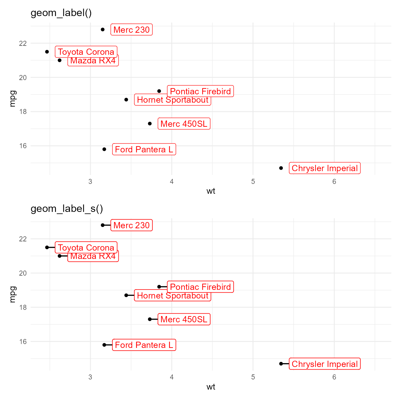
(p + geom_label(colour = "red",
                border.colour = "black",
                nudge_x = 0.1, hjust = 0) + labs(title = "geom_label()")) /
  (p + geom_label_s(colour = "red",
                    colour.target = "text",
                nudge_x = 0.1, hjust = 0) + labs(title = "geom_label_s()"))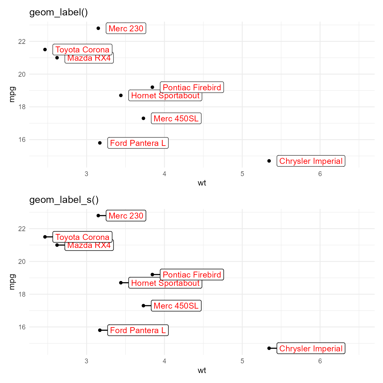
(p + geom_label(colour = "red",
                border.colour = "darkgreen",
                nudge_x = 0.1, hjust = 0)
 + labs(title = "geom_label()")) /
  (p + geom_label_s(colour = "red",
                    default.colour = "darkgreen",
                    colour.target = "text",
                    nudge_x = 0.1, hjust = 0))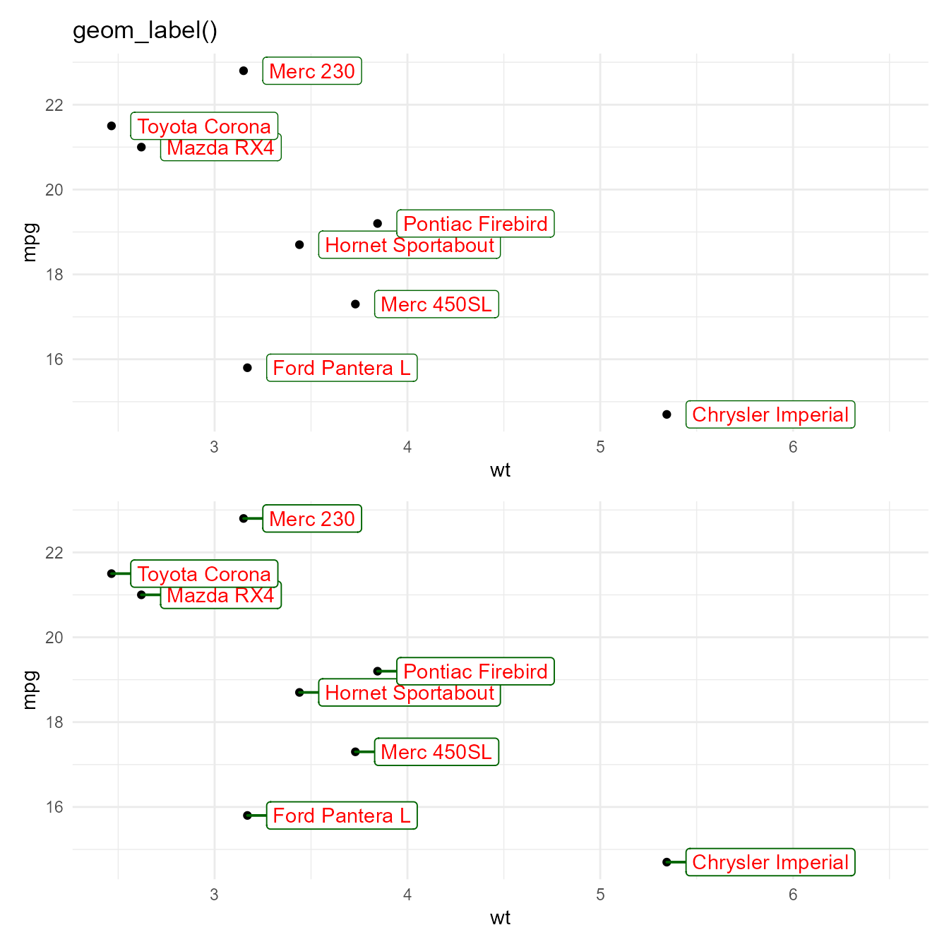
update_theme(geom = element_geom(colour = "red"))

(p + geom_label(nudge_x = 0.1, hjust = 0) + labs(title = "geom_label()")) /
  (p + geom_label_s(nudge_x = 0.1, hjust = 0) + labs(title = "geom_label_s()"))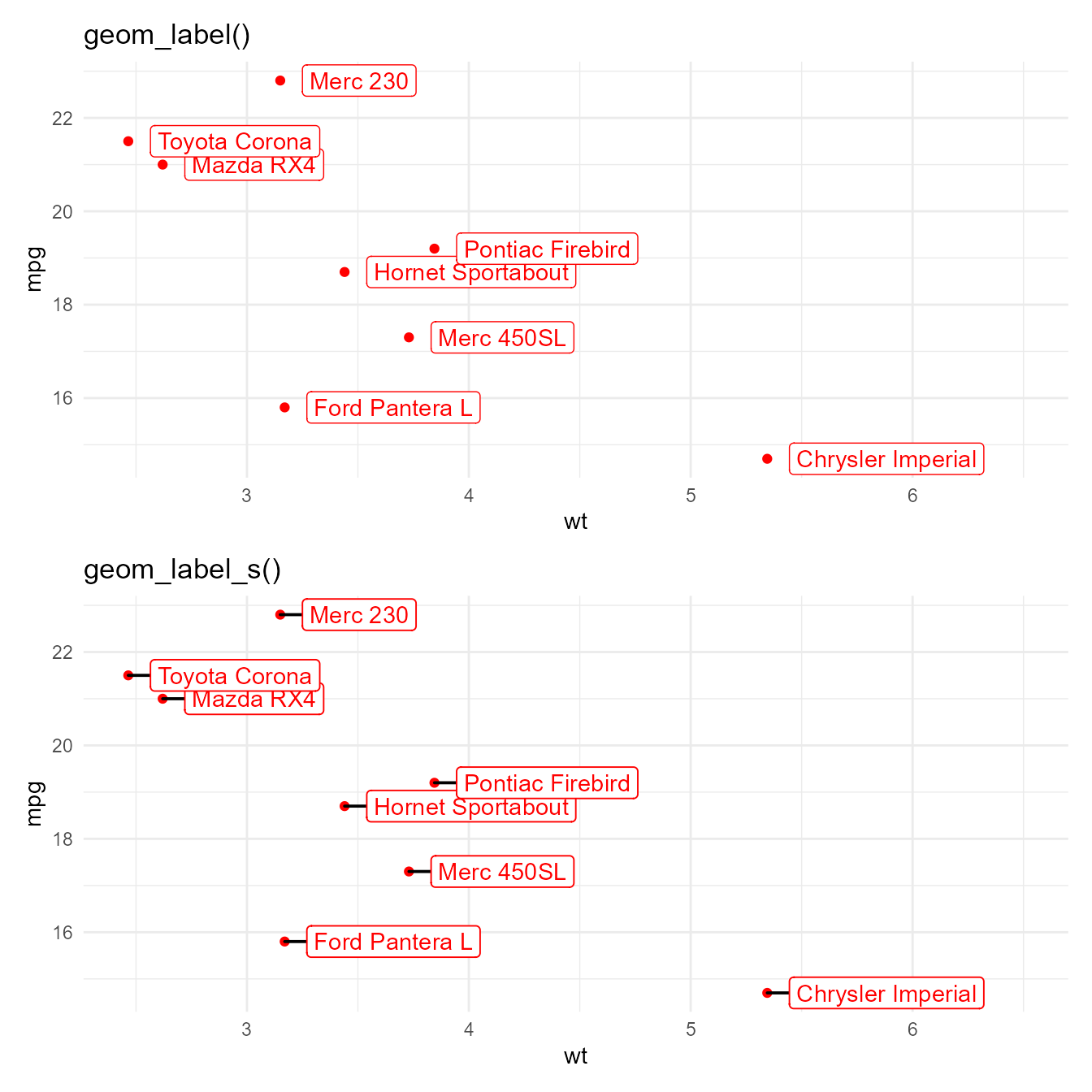
update_theme(geom = element_geom(colour = "black", borderwidth = 1.5))

(p + geom_label(nudge_x = 0.1, hjust = 0) + labs(title = "geom_label()")) /
  (p + geom_label_s(nudge_x = 0.1, hjust = 0) + labs(title = "geom_label_s()"))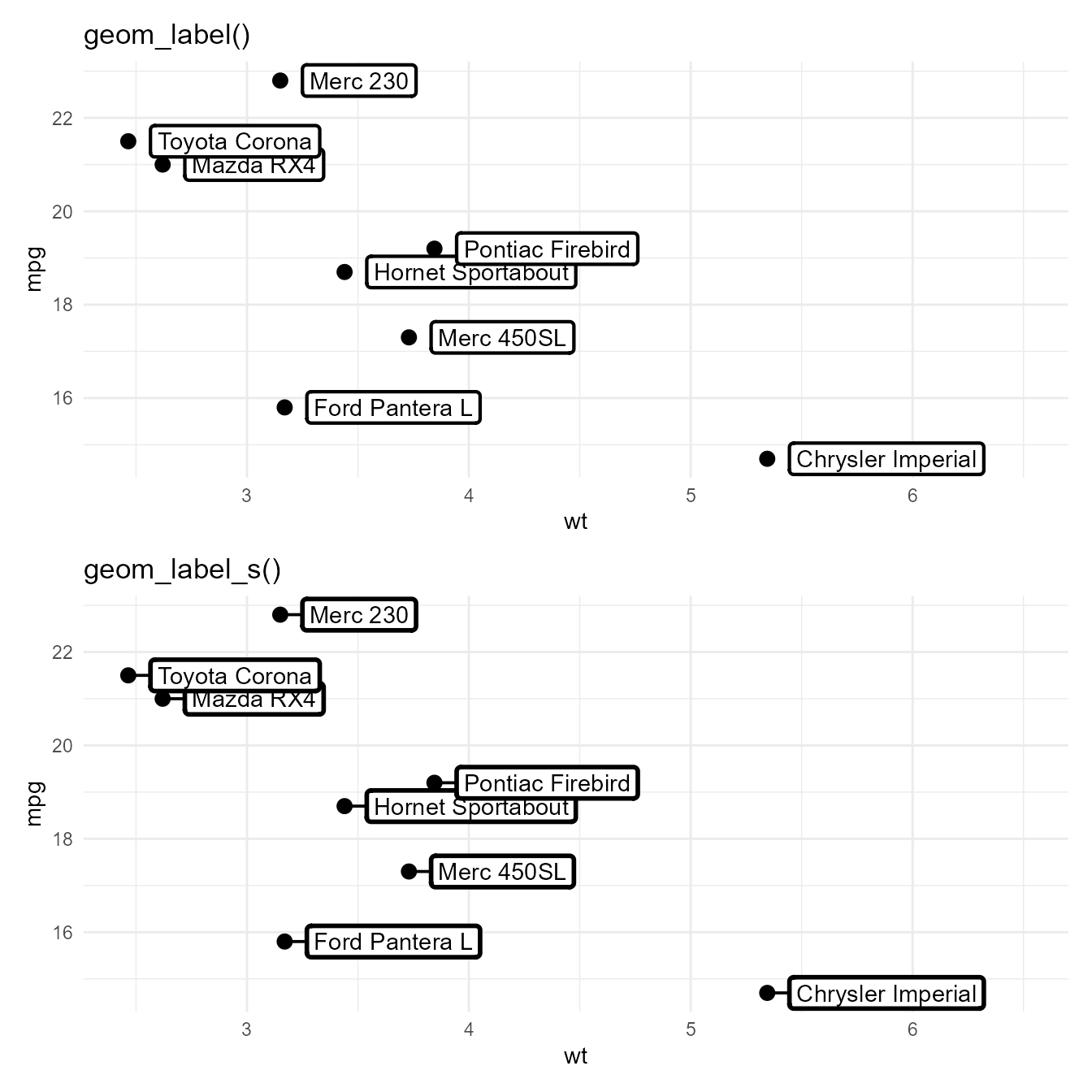
update_theme(geom = element_geom(colour = "black"))
(p + geom_label(linewidth = 0,
                nudge_x = 0.1, hjust = 0) + labs(title = "geom_label()")) /
  (p + geom_label_s(linewidth = 0,
                    nudge_x = 0.1, hjust = 0) + labs(title = "geom_label_s()"))
opts_chunk$set(fig.align = 'center',
               fig.show = 'hold', fig.width = 7, fig.height = 4)
set_theme(theme_minimal())
update_theme(geom = element_geom(ink = "blue"))
p + geom_label_s(colour = "red", colour.target = "text",
                 nudge_x = 0.1, hjust = 0)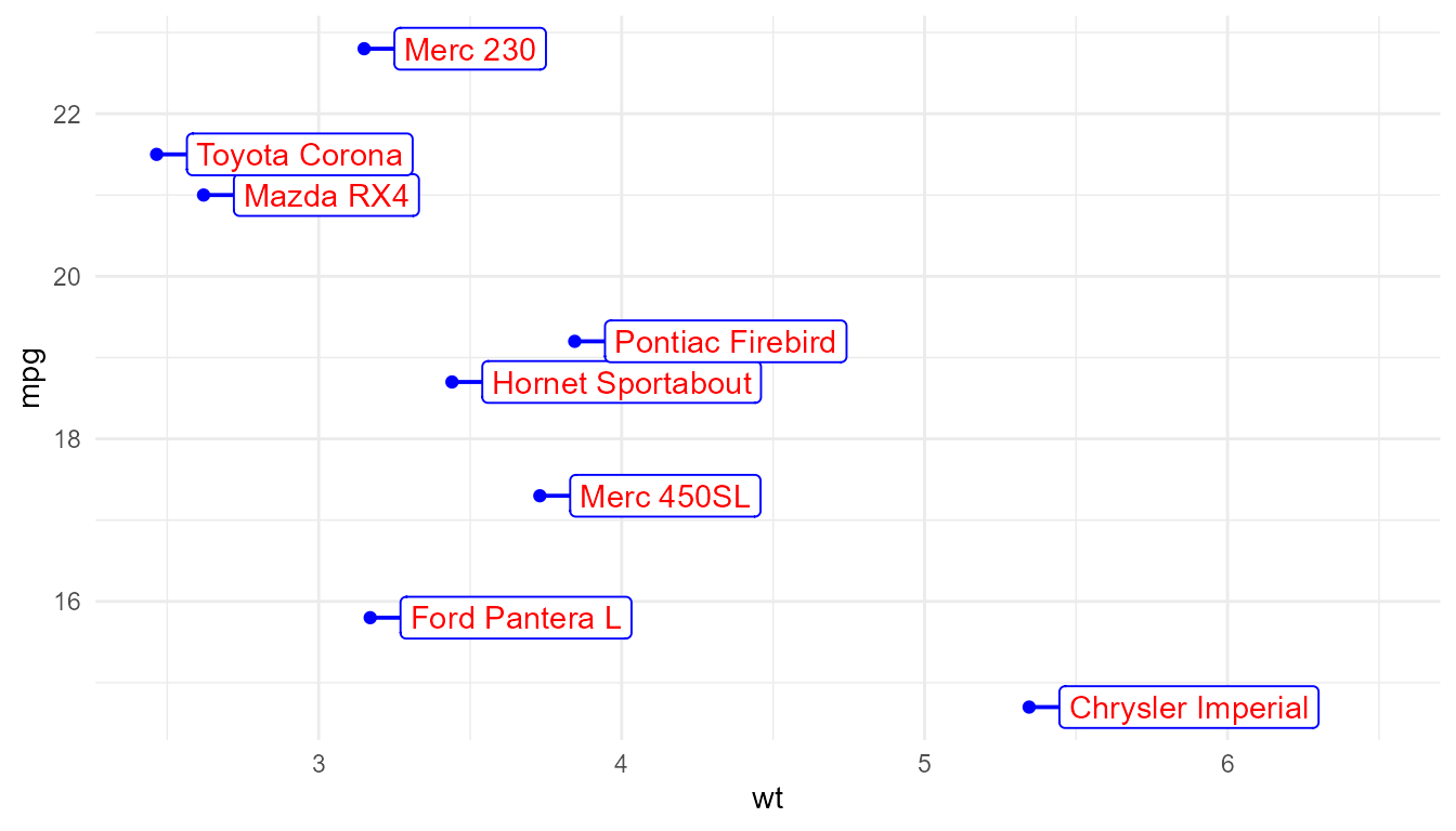
set_theme(theme_minimal() +
  theme(geom = element_geom(ink = "blue")))

p +
  geom_label_s(colour = "red",
               colour.target = "text",
               nudge_x = 0.1, hjust = 0)
set_theme(theme_minimal())

p +
  geom_label_s(colour = "red",
               default.colour = "blue",
               colour.target = "text",
               nudge_x = 0.1, hjust = 0)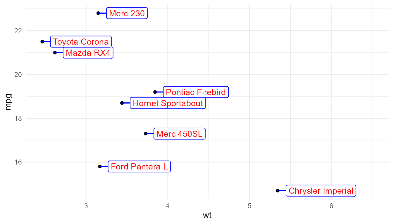
If the connecting segment has an arrow head, it is also targetted as
a component of the "segment".
set_theme(theme_minimal())

p +
  geom_label_s(colour = "red",
               colour.target = "segment",
               arrow = grid::arrow(length = unit(2, "mm")),
               point.padding = 1,
               nudge_x = 0.25, hjust = 0)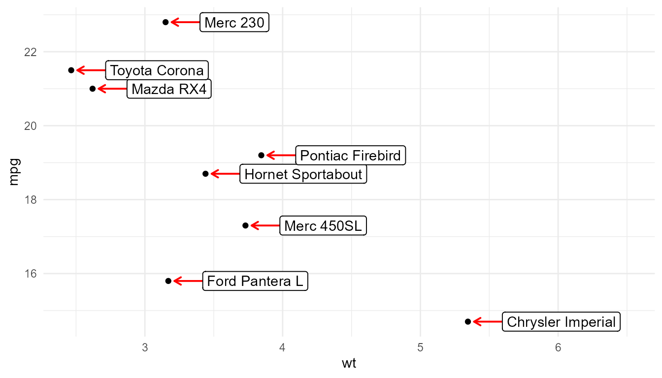
set_theme(theme_minimal())

p +
  geom_label_s(colour = "red",
               default.colour = "blue",
               colour.target = c("box.line", "segment"),
               nudge_x = 0.1, hjust = 0)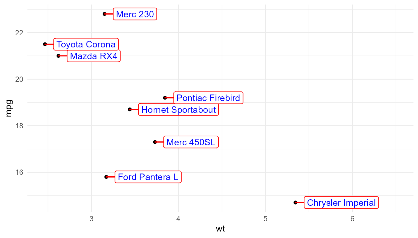
geom_table
p1 + annotate(geom = "table",
              colour = "red",
              label = data.frame(a = 1:2, b = 3:4),
              x = 6, y = 22)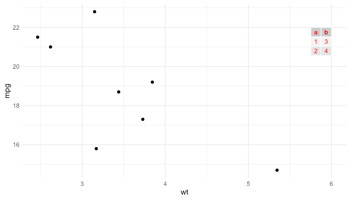
p1 + annotate(geom = "table",
              colour = "red",
              colour.target = "table.rules",
              label = data.frame(a = 1:2, b = 3:4),
              x = 6, y = 22)
p1 + annotate(geom = "table",
              colour = "red",
              colour.target = "all",
              label = data.frame(a = 1:2, b = 3:4),
              x = 6, y = 22)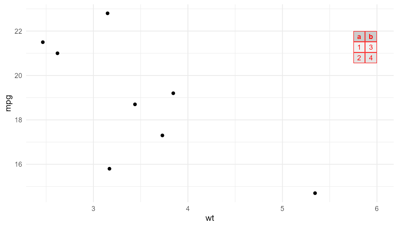
p1 + annotate(geom = "table",
              colour = "red",
              colour.target = "none",
              label = data.frame(a = 1:2, b = 3:4),
              x = 6, y = 22)