Test with Ander's hourly and Titta's greenhouse spectra
Package ‘rYoctoPuceInOut’ 0.0.1.9001
Pedro J. Aphalo
2026-02-08
Source:vignettes/articles/simul-calibration.Rmd
simul-calibration.RmdSet up
This article is not part of the package, it is a on-line-only supplementary article. It depends on R packages not included as imports or suggests of ‘rYoctoPuceInOut’. To run the examples below it can be necessary to install one or more of the packages attached in this code chunk.
AS7343 spectral response
The AS7343 sensor has 13 channels covering wavelengths in the range 370-900 nm.
ams_AS7343.mspct <- subset2mspct(sensors.mspct$ams_AS7343)
autoplot(ams_AS7343.mspct)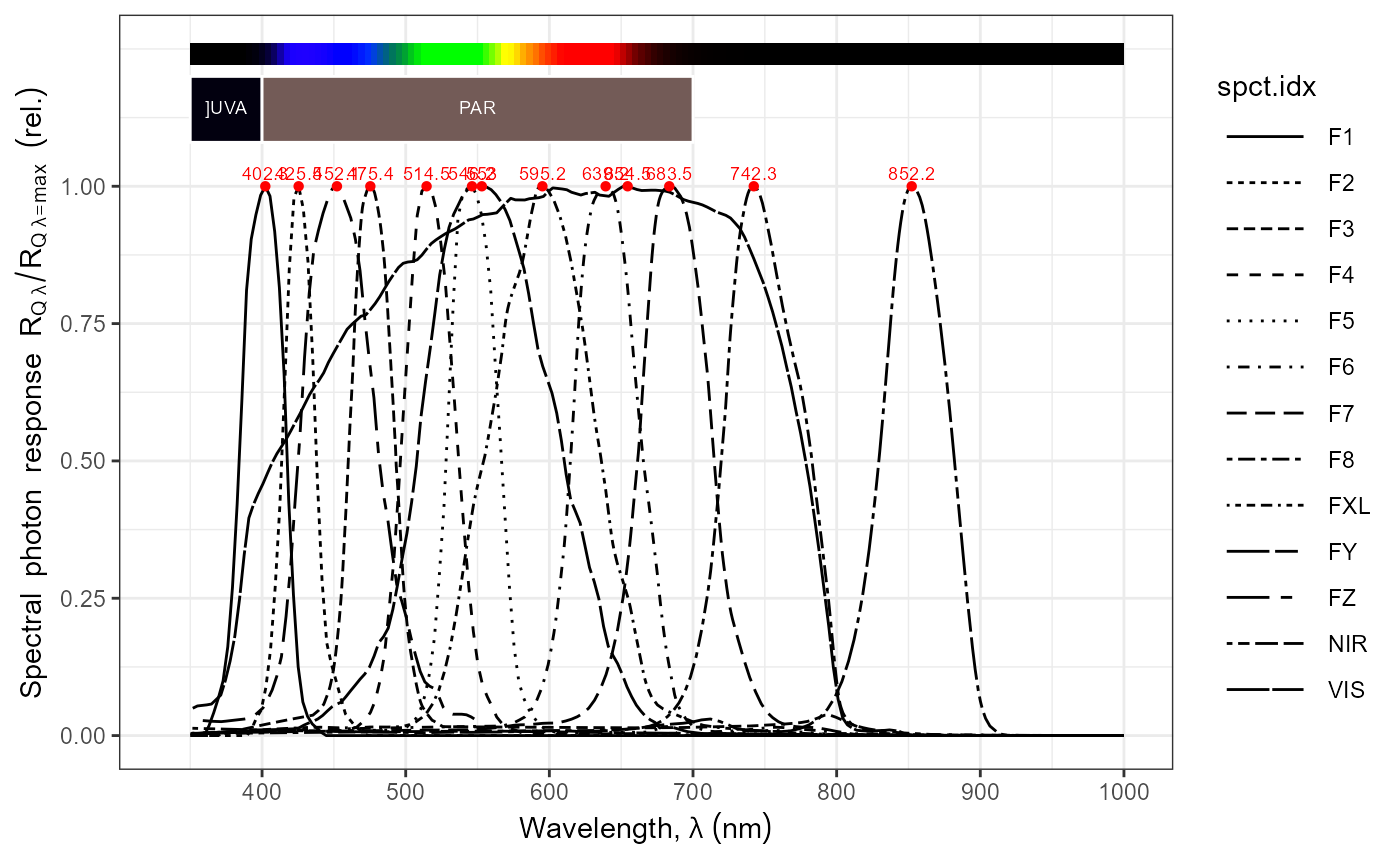
autoplot(ams_AS7343.mspct, norm = "undo")## Normalization 'norm = skip' applied before plotting."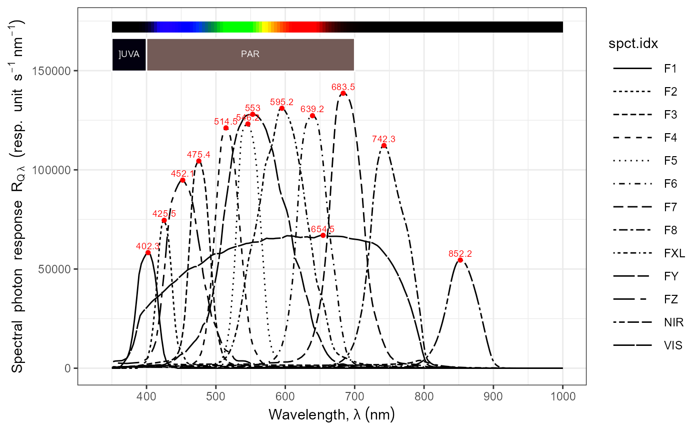
Hourly sunlight spectra
load("data/kumpula-all-hourly-mspct-anders-lindfors.rda")
test.hourly.mspct <- all_hourly.mspct
length(all_hourly.mspct)
## [1] 11768Simulated calibration
With a list of waveband objects we can compute multiple
irradiances by integrating the radiation spectrum over multiple ranges
of wavelengths.
extra.wavebands <-
  c(Plant_bands("Sellaro"),
    list(Red("Smith20"), Far_red("Smith20")))
Compute irradiances
irradiances.tb <-
  xPAR_irrad(test.mspct,
             w.band = Plant_bands("Sellaro"),
             scale.factor = 1e6, # mol m-2 s-1 -> umol m-2 s-1
             return.tb = TRUE)
nrow(irradiances.tb)
## [1] 124
ncol(irradiances.tb)## [1] 13
channels.ls <-list()
spct.names <- names(test.mspct)
for (name in spct.names) {
#  print(name)
  temp.tb <-
    simul_sensor_response(test.mspct[[name]][ , 1:2],
                         sensors.mspct[["ams_AS7343"]],
                         norm = "undo")
  channels.ls[[name]] <- temp.tb[[2]]
}
channels.tb <- as.data.frame(t(as.data.frame(channels.ls)))
colnames(channels.tb) <- temp.tb[["spct.idx"]]
channels.tb[["spct.idx"]] <- spct.names
It is safer to join the irradiance and sensor response data matching rows by spectrum name than by position.
colnames(irradiances.tb)## [1] "spct.idx" "Q_xPAR" "Q_ePAR" "Q_PAR"
## [5] "Q_FR.700.750" "Q_UVB.ISO" "Q_UVA2.CIE" "Q_UVA1.CIE"
## [9] "Q_Blue.Sellaro" "Q_Green.Sellaro" "Q_Red.Sellaro" "Q_FarRed.Sellaro"
## [13] "Q_]UVB.ISO"
colnames(channels.tb)## [1] "F1" "F2" "F3" "F4" "F5" "F6"
## [7] "F7" "F8" "FXL" "FY" "FZ" "NIR"
## [13] "VIS" "spct.idx"
all_data.tb <- right_join(irradiances.tb, channels.tb)## Joining with `by = join_by(spct.idx)`
## Joining with `by = join_by(spct.idx)`
PfrPtot <- numeric()
idx <- 0
spct.names <- names(test.mspct)
for (name in spct.names) {
  idx <- idx + 1L
#  print(name)
  PfrPtot[idx] <- Pfr_Ptot(test.mspct[[name]][ , 1:2])
}
all_data.tb[["Pfr.Ptot"]] <- PfrPtot
save(all_data.tb, file = "data/all-hourly-summaries.rda")PAR
The first question is: Is the VIS channel corrected with FR channel FF8 a good enough match to be used for PAR measurements?
ggplot(all_data.tb, aes(Q_PAR, VIS - 0.45 * F8)) +
  geom_point(alpha = my.default.alpha) +
  stat_poly_line(formula = y ~ x + 0, method = "sma") +
  stat_poly_eq(use_label("eq", "R2", "n", "AIC"),
               formula = y ~ x + 0, method = "sma")
## SMA/MA, band is currently for slope only!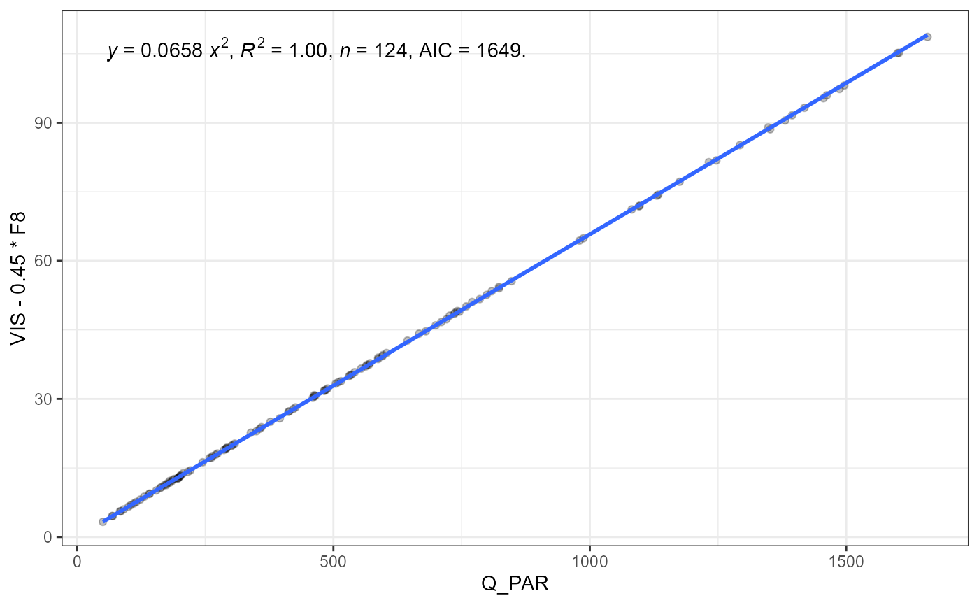
ePAR
Would it also work for ePAR?
ggplot(all_data.tb, aes(Q_ePAR, VIS)) +
  geom_point(alpha = my.default.alpha) +
  stat_poly_line(formula = y ~ x + 0, method = "sma") +
  stat_poly_eq(use_label("eq", "R2", "n", "AIC"),
               formula = y ~ x + 0, method = "sma")
## SMA/MA, band is currently for slope only!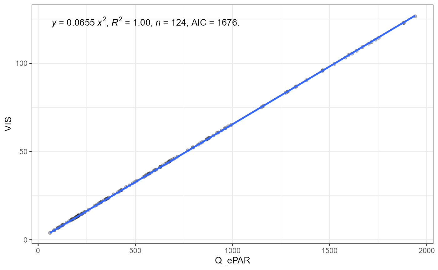
For sunlight the answer to both questions is: yes.
UVA1
In the case of UVA1, the centre wavelength of the nearest sensor channel is about 20 nm too long. Although R^2 remains very high there is more variation around the “calibration” line than for PAR or ePAR.
ggplot(all_data.tb, aes(Q_UVA1.CIE, F1 - 0.29 * F2)) +
  geom_point(alpha = my.default.alpha) +
  stat_poly_line(formula = y ~ x, method = "sma") +
  stat_poly_eq(use_label("eq", "R2", "n", "AIC"),
               formula = y ~ x, method = "sma",
               size = 2.7)
## SMA/MA, band is currently for slope only!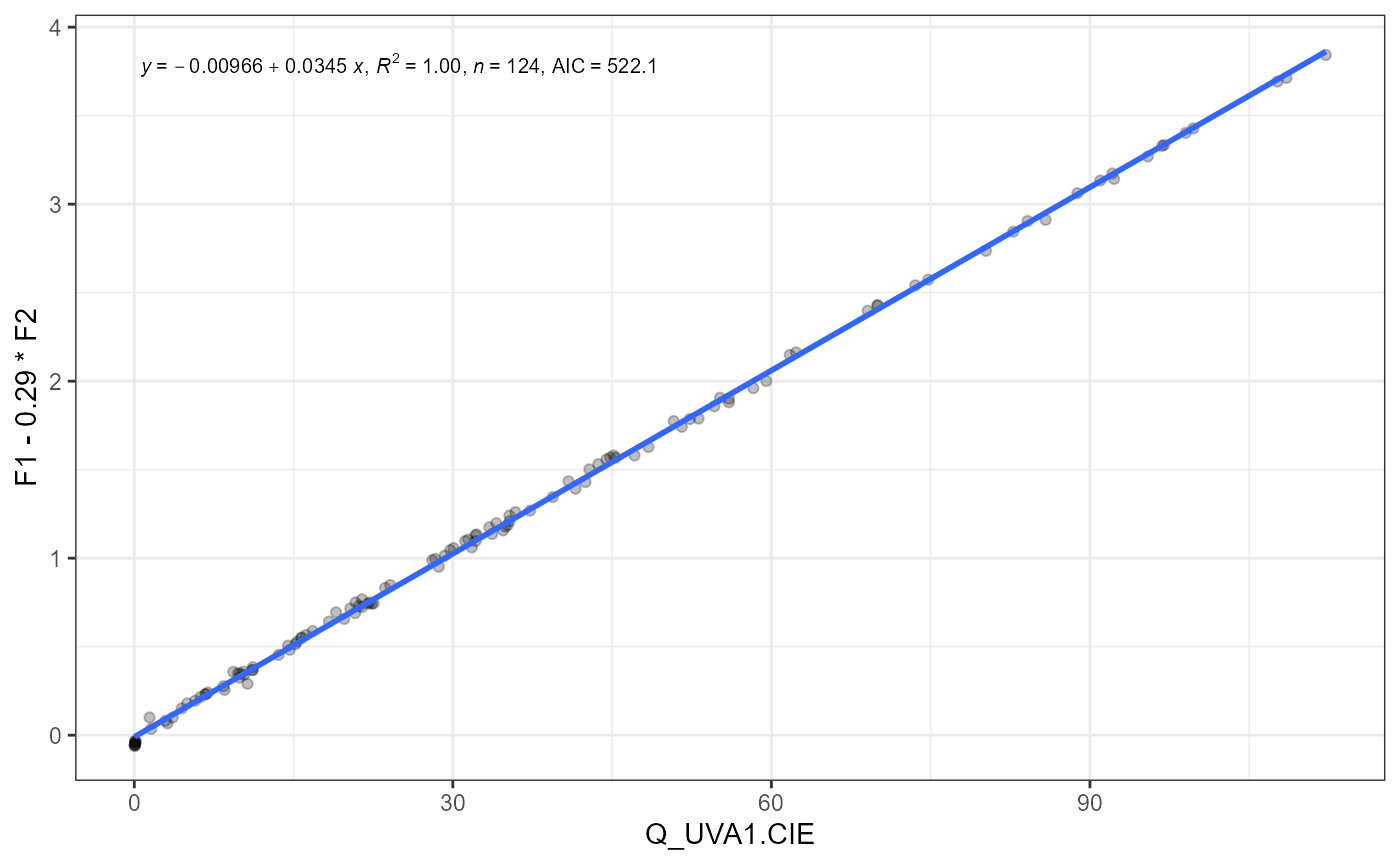
UVA1:PAR photon ratio
ggplot(all_data.tb, aes(Q_UVA1.CIE / Q_PAR, (F1 - 0.29 * F2) / VIS)) +
  geom_point(alpha = my.default.alpha) +
  stat_poly_line(formula = y ~ x, method = "sma") +
  stat_poly_eq(use_label("eq", "R2", "n", "AIC"),
               formula = y ~ x, method = "sma",
               size = 2.7)
## SMA/MA, band is currently for slope only!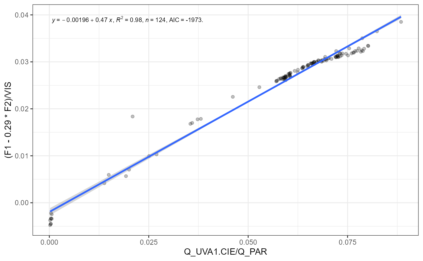
Blue
ggplot(all_data.tb, aes(Q_Blue.Sellaro, F2 + 0.29 * F3)) +
  geom_point(alpha = my.default.alpha) +
  stat_poly_line(formula = y ~ x + 0, method = "sma") +
  stat_poly_eq(use_label("eq", "R2", "n", "AIC"),
               formula = y ~ x + 0, method = "sma")
## SMA/MA, band is currently for slope only!
Green
ggplot(all_data.tb, aes(Q_Green.Sellaro, 0.47 * F4 + F5)) +
  geom_point(alpha = my.default.alpha) +
  stat_poly_line(formula = y ~ x + 0, method = "sma") +
  stat_poly_eq(use_label("eq", "R2", "n", "AIC"),
               formula = y ~ x + 0, method = "sma")
## SMA/MA, band is currently for slope only!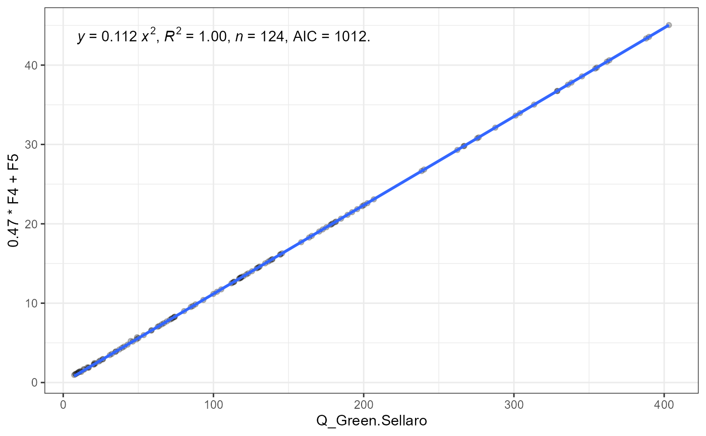
B:G photon ratio
ggplot(all_data.tb, aes(Q_Blue.Sellaro / Q_Green.Sellaro,
                        (F2 + 0.29 * F3) / (0.47 * F4 + F5))) +
  geom_point(alpha = my.default.alpha) +
  stat_poly_line(formula = y ~ x, method = "sma") +
  stat_poly_eq(use_label("eq", "R2", "n", "AIC"),
               formula = y ~ x, method = "sma",
               size = 2.7)
## SMA/MA, band is currently for slope only!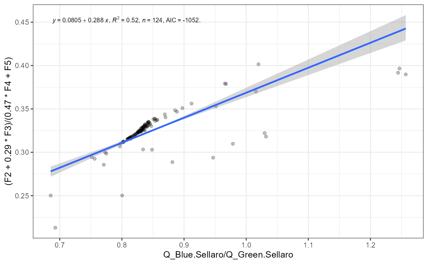
Red
ggplot(all_data.tb, aes(Q_Red.Sellaro, F6 - 0.3 * F5)) +
  geom_point(alpha = my.default.alpha) +
  stat_poly_line(formula = y ~ x + 0, method = "sma") +
  stat_poly_eq(use_label("eq", "R2", "n", "AIC"),
               formula = y ~ x + 0, method = "sma")
## SMA/MA, band is currently for slope only!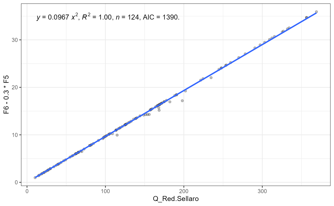
Far Red
ggplot(all_data.tb, aes(Q_FarRed.Sellaro, F8)) +
  geom_point(alpha = my.default.alpha) +
  stat_poly_line(formula = y ~ x + 0, method = "sma") +
  stat_poly_eq(use_label("eq", "R2", "n", "AIC"),
               formula = y ~ x + 0, method = "sma")
## SMA/MA, band is currently for slope only!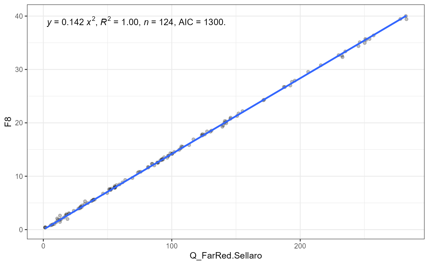
FR:R+FR photon fraction
ggplot(all_data.tb, aes(Q_FarRed.Sellaro / (Q_FarRed.Sellaro + Q_Red.Sellaro), F8 / (F6 - 0.3 * F5 + F8))) +
  geom_point(alpha = my.default.alpha) +
  stat_poly_line(formula = y ~ x + I(x^2), method = "lm") +
  stat_poly_eq(use_label("eq", "R2", "n", "AIC"),
               formula = y ~ x + I(x^2), method = "lm",
               size = 2.7)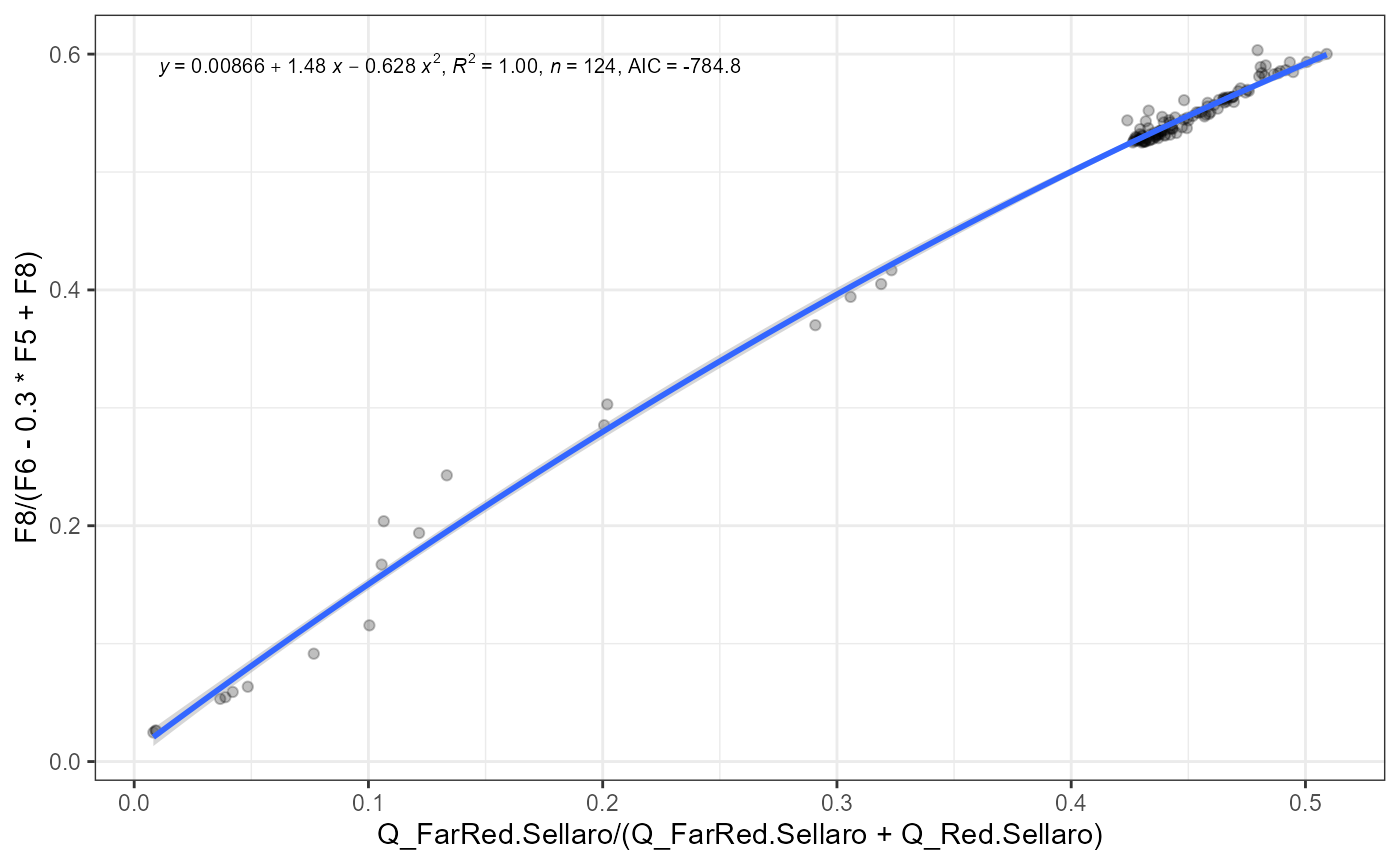
The range of meaningful values for R:FR in sunlight is narrow and consequently small errors in the quantification of R and/or FR irradiance result in R:FR errors that can be thought as important for plant responses. Possibly, more important, is that the R:FR photon ratio measured based on different waveband definitions is not consistent in sunlight.
The choice of wavebands is rather arbitrary as the Pfr:Ptot fraction depends on a broad range of wavelengths and different wavelengths affect it with different weights.
FR:ePAR photon fraction
ggplot(all_data.tb, aes(Q_FarRed.Sellaro / Q_ePAR, F8 / VIS)) +
  geom_point(alpha = my.default.alpha) +
  stat_poly_line(formula = y ~ x + I(x^2), method = "lm") +
  stat_poly_eq(use_label("eq", "R2", "n", "AIC"),
               formula = y ~ x + I(x^2), method = "lm",
               size = 2.7)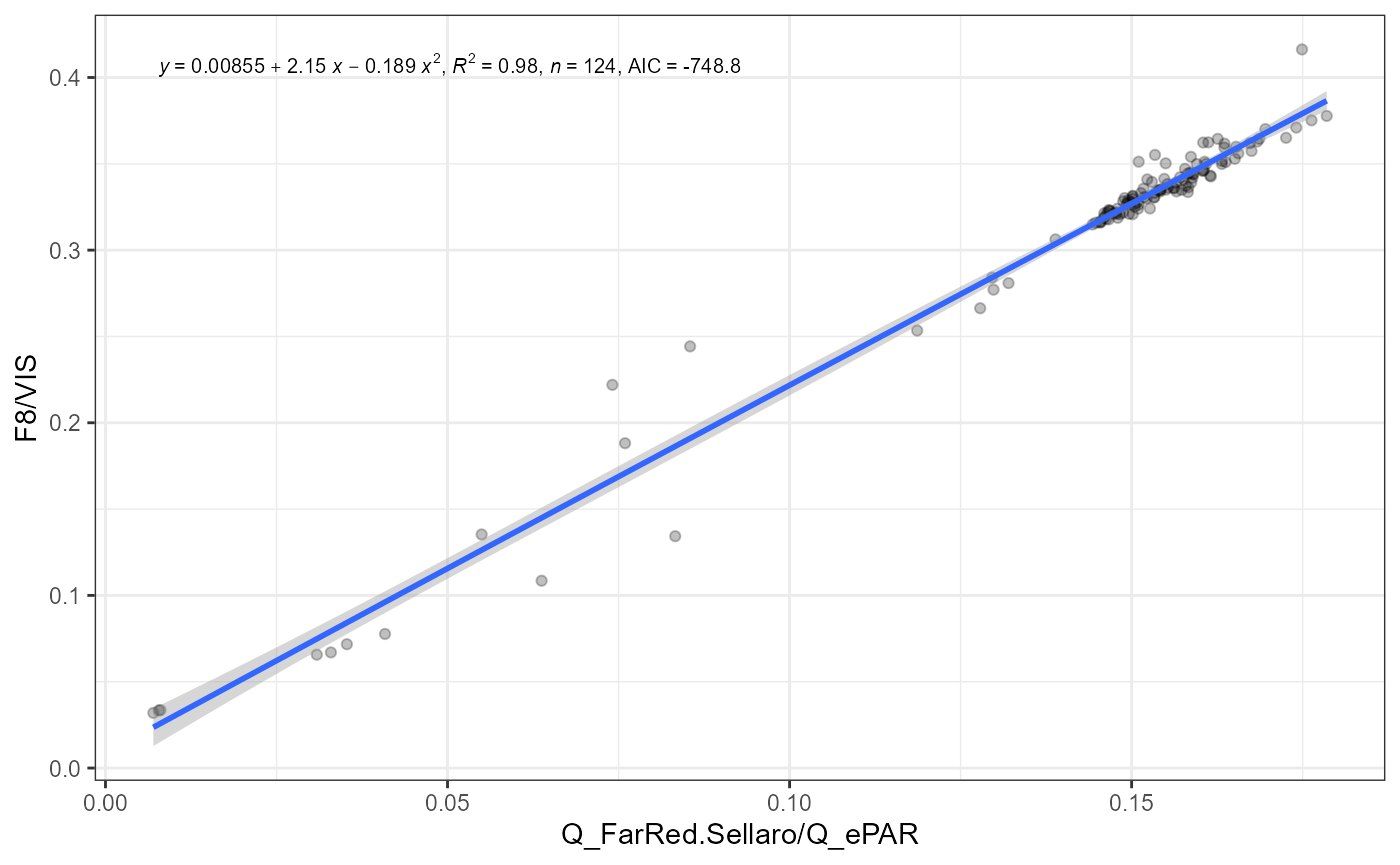
FR:PAR photon fraction
ggplot(all_data.tb,
       aes(Q_FarRed.Sellaro / Q_PAR, F8 / (VIS - 0.45 * F8))) +
  geom_point(alpha = my.default.alpha) +
  stat_poly_line(formula = y ~ x + I(x^2), method = "lm") +
  stat_poly_eq(use_label("eq", "R2", "n", "AIC"),
               formula = y ~ x + I(x^2), method = "lm",
               size = 2.7)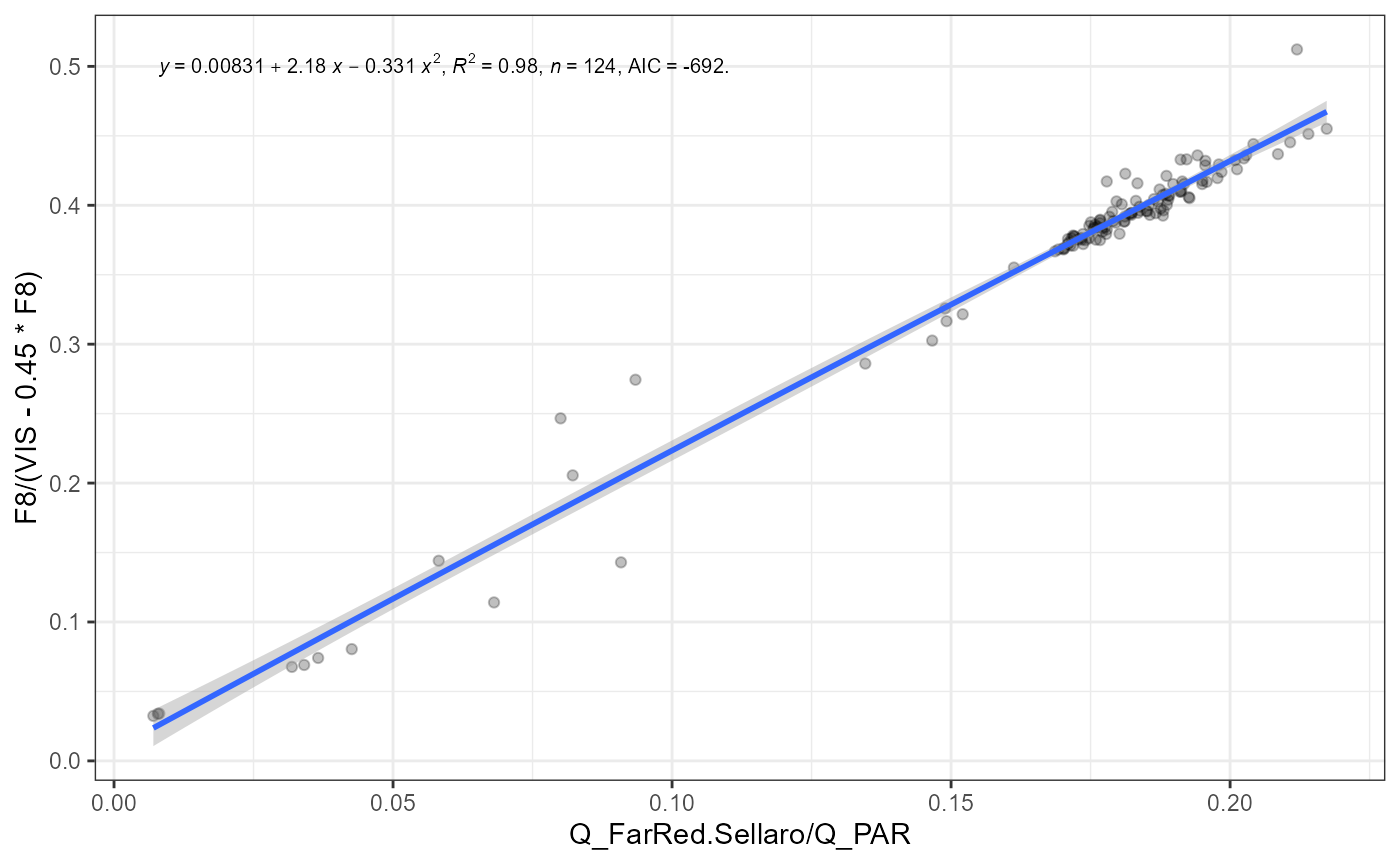
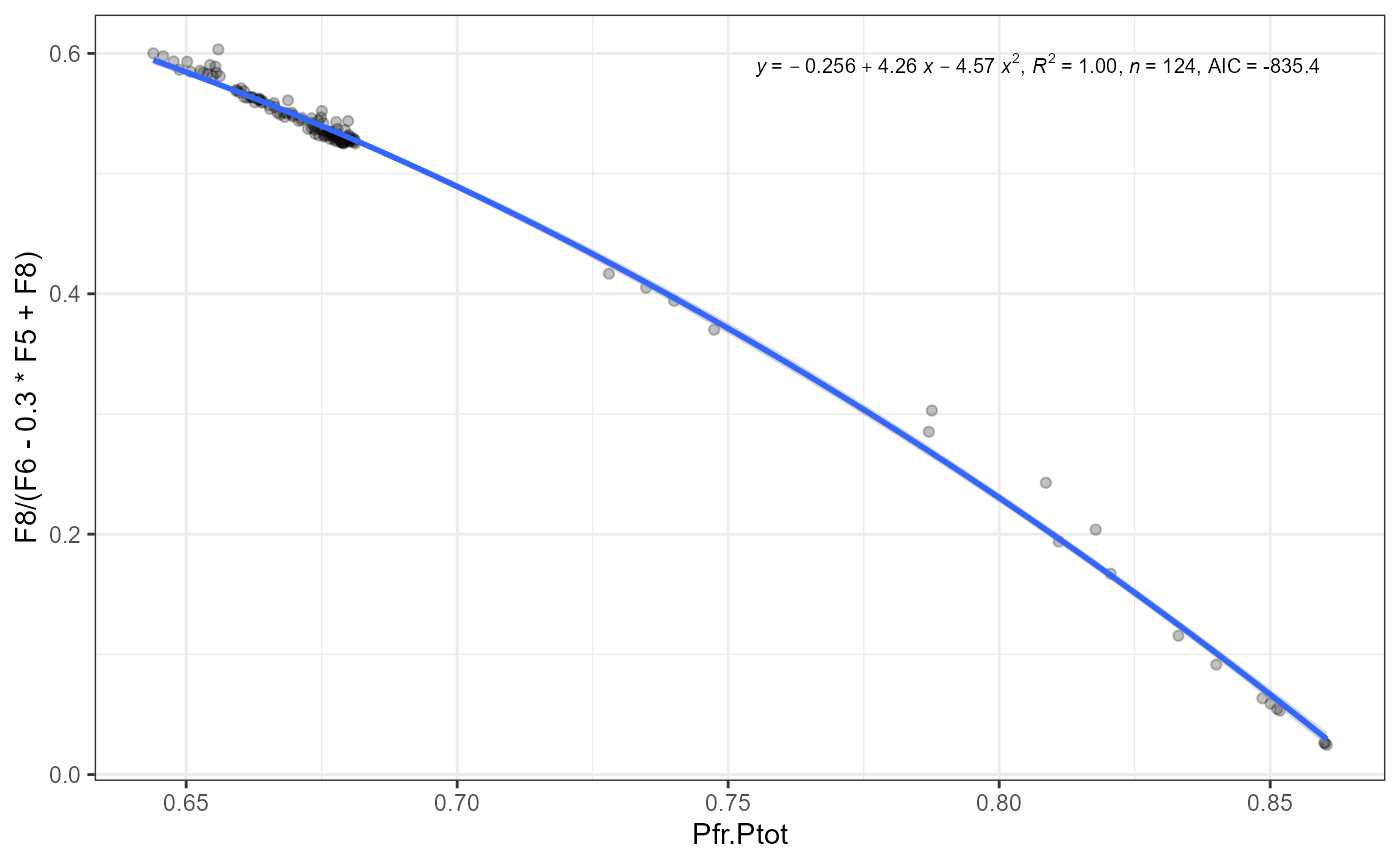
Pfr:Ptot vs. FR fraction
ggplot(all_data.tb, aes(Pfr.Ptot,
                        Q_FarRed.Sellaro / (Q_FarRed.Sellaro + Q_Red.Sellaro))) +
  geom_point(alpha = my.default.alpha) +
  stat_poly_line(formula = y ~ x, method = "sma") +
  stat_poly_eq(use_label("eq", "R2", "n", "AIC"),
               label.x = "right",
               formula = y ~ x, method = "sma")
## SMA/MA, band is currently for slope only!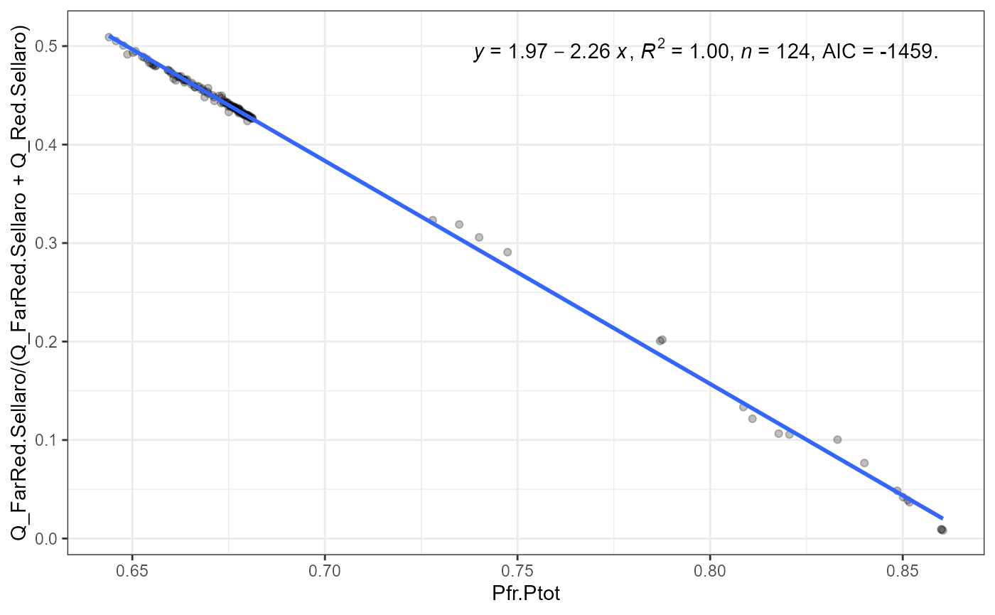
ggplot(all_data.tb, aes(Pfr.Ptot, F8 / (F6 - 0.3 * F5 + F8))) +
  geom_point(alpha = my.default.alpha) +
  stat_poly_line(formula = y ~ x + I(x^2), method = "lm") +
  stat_poly_eq(use_label("eq", "R2", "n", "AIC"),
               label.x = "right",
               formula = y ~ x + I(x^2), method = "lm",
               size = 2.7)