geom_table and geom_table_npc add data frames as table insets
to the base ggplot, using syntax similar to that of
geom_text and geom_text_s. In most
respects they behave as any other ggplot geometry: they add a layer
containing one or more grobs and grouping and faceting works as usual. The
most common use of geom_table is to add data labels that are whole
tables rather than text. geom_table_npc is used to add tables
as annotations to plots, but contrary to layer function annotate,
geom_table_npc is data driven and respects grouping and facets,
thus plot insets can differ among panels.
Usage
geom_table(
  mapping = NULL,
  data = NULL,
  stat = "identity",
  position = "identity",
  ...,
  nudge_x = 0,
  nudge_y = 0,
  default.colour = NA,
  default.color = default.colour,
  colour.target = "table.text",
  color.target = colour.target,
  default.alpha = 1,
  alpha.target = "all",
  fontsize.scaling = 0.825,
  add.segments = TRUE,
  box.padding = 0.25,
  point.padding = 1e-06,
  segment.linewidth = 0.5,
  min.segment.length = 0,
  arrow = NULL,
  table.theme = NULL,
  table.rownames = FALSE,
  table.colnames = TRUE,
  table.hjust = 0.5,
  parse = FALSE,
  na.rm = FALSE,
  show.legend = FALSE,
  inherit.aes = FALSE
)

geom_table_npc(
  mapping = NULL,
  data = NULL,
  stat = "identity",
  position = "identity",
  ...,
  default.colour = NA,
  default.color = default.colour,
  colour.target = "table.text",
  color.target = colour.target,
  default.alpha = 1,
  alpha.target = "all",
  fontsize.scaling = 0.825,
  table.theme = NULL,
  table.rownames = FALSE,
  table.colnames = TRUE,
  table.hjust = 0.5,
  parse = FALSE,
  na.rm = FALSE,
  show.legend = FALSE,
  inherit.aes = FALSE
)
Arguments
- mapping
The aesthetic mapping, usually constructed with
aes. Only needs to be set at the layer level if you are overriding the plot defaults.- data
A layer specific dataset - only needed if you want to override the plot defaults.
- stat
The statistical transformation to use on the data for this layer, as a string.
- position
Position adjustment, either as a string, or the result of a call to a position adjustment function.
- ...
other arguments passed on to
layer. This can include aesthetics whose values you want to set, not map. Seelayerfor more details.- nudge_x, nudge_y
Horizontal and vertical adjustments to nudge the starting position of each "label". The units for
nudge_xandnudge_yare the same as for the data units on the x-axis and y-axis.- default.colour, default.color
A colour definition to use for elements not targeted by the colour aesthetic. If
NAthe colours in the table theme are not modified.- colour.target, color.target
A vector of character strings with one or more of
"all","table","table.text","table.rules","segment"or"none".- default.alpha
numeric in [0..1] A transparency value to use for elements not targeted by the alpha aesthetic. If
NAthe alpha channel of the colour definitions is not modified.- alpha.target
A vector of character strings with one or more of
"all","table","table.text","table.rules"and"table.canvas","segment"or"none".- fontsize.scaling
A scaling factor to apply to the size aesthetic retrieved from the theme or mapped, applied to table text.
- add.segments
logical Display connecting segments or arrows between original positions and displaced ones if both are available.
- box.padding, point.padding
numeric By how much each end of the segments should shortened in mm.
- segment.linewidth
numeric Width of the segments or arrows in mm.
- min.segment.length
numeric Segments shorter that the minimum length are not rendered, in mm.
- arrow
specification for arrow heads, as created by
arrow- table.theme
NULL, list or function A gridExtra ttheme defintion, or a constructor for a ttheme or NULL for default. If
nULLthe theme is retrieved from R optionat the time the plot is rendered.- table.rownames, table.colnames
logical flag to enable or disable printing of row names and column names.
- table.hjust
numeric Horizontal justification for the core and column headings of the table.
- parse
If TRUE, the labels will be parsed into expressions and displayed as described in
?plotmath.- na.rm
If
FALSE(the default), removes missing values with a warning. IfTRUEsilently removes missing values.- show.legend
logical. Should this layer be included in the legends?
NA, the default, includes if any aesthetics are mapped.FALSEnever includes, andTRUEalways includes.- inherit.aes
If
FALSE, overrides the default aesthetics, rather than combining with them. This is most useful for helper functions that define both data and aesthetics and shouldn't inherit behaviour from the default plot specification, e.g.borders.
Details
geom_table and geom_table_npc expect a list of data frames
("data.frame" class or derived) to be mapped to the label
aesthetic. These geoms work with tibbles or data frames as data as
they both support list objects as member variables.
A table is built with function gridExtra::gtable for each
data frame in the list, and formatted according to a ttheme (table
theme) list object or ttheme constructor function passed as argument
to parameter table.theme. If the value passed as argument to
table.theme is NULL the table theme used is that set as
default through R option ggpmisc.ttheme.default at the time the plot
is rendered or the ttheme_gtdefault constructor function if
not set.
If the argument passed to table.theme or set through R option
ggpmisc.ttheme.default is a constructor function (passing its name
without parenthesis), the values mapped to size, colour,
fill, alpha, and family aesthetics will the passed to
this theme constructor for each individual table. In contrast, if a ready
constructed ttheme stored as a list object is passed as argument
(e.g., by calling the constructor, using constructor name followed by
parenthesis), it is used as is, with mappings to aesthetics colour,
fill, alpha, and family ignored if present. By default
the constructor ttheme_gtdefault is used and colour and
fill, are mapped to NA. Mapping these aesthetics to NA
triggers the use the values set in the ttheme. As the table is built
with function gridExtra::gtable(), for details, please, consult
tableGrob and ttheme_gtdefault.
The character strings in the data frame can be parsed into R expressions so
the inset tables can include maths. With parse = TRUE parsing is
attempted on each table cell, but failure triggers fall-back to rendering
without parsing, on a cell by cell basis. Thus, a table can contain a
mixture cells and/or headings that require parsing or not (see the
documentation in gridExtra-package for details).
The x and y aesthetics determine the position of the whole
inset table, similarly to that of a text label, justification is
interpreted as indicating the position of the inset table with respect to
its horizontal and vertical axes (rows and columns in the
data frame), and angle is used to rotate the inset table as a whole.
The default for the colour and fill aesthetics is to retrieve
them from the table theme, while family and size are
retrieved from the geom element of the ggplot theme.
Of these two geoms only geom_table supports the plotting of
connecting segments or arrows when its position has been modified by a
position function. This is because geom_table_npc uses
a coordinate system that is unrelated to data units, scales or data in
other plot layers. In the case of geom_table_npc, npcx and
npcy pseudo-aesthetics determine the position of the inset table. By
default, hjust and vjust are set to "inward" to avoid
clipping at the edge of the plot canvas.
Note
Complex tables with annotations or different colouring of rows or cells
can be constructed with functions in package 'gridExtra' or in any other
way as long as they can be saved as grid graphical objects and then added
to a ggplot as a new layer with geom_grob.
Alignment
You can modify text alignment with the vjust and
hjust aesthetics. These can either be a number between 0
(right/bottom) and 1 (top/left) or a character ("left",
"middle", "right", "bottom", "center",
"top"). In addition, you can use special alignments for
justification including "position", "inward" and
"outward". Inward always aligns text towards the center of the
plotting area, and outward aligns it away from the center of the plotting
area. If tagged with _mean or _median (e.g.,
"outward_mean") the mean or median of the data in the panel along
the corresponding axis is used as center. If the characters following the
underscore represent a number (e.g., "outward_10.5") the reference
point will be this value in data units. Position justification is computed
based on the direction of the displacement of the position of the label so
that each individual text or label is justified outwards from its original
position. The default justification is "position".
If no position displacement is applied, or a position function defined in
'ggplot2' is used, these geometries behave similarly to the corresponding
ones from package 'ggplot2' with a default justification of 0.5 and
no segment drawn.
Position functions
Many layer functions from package 'ggpp' are
designed to work seamlessly with position functions that keep, rather than
discard, the original x and y positions in data when
computing a new displaced position. See position_nudge_keep,
position_dodge_keep, position_jitter_keep,
position_nudge_center, position_nudge_line,
position_nudge_to, position_dodgenudge,
position_jitternudge, and position_stacknudge
for examples and details of their use.
Plot boundaries and clipping
The "width" and "height" of an inset as for a text element are 0, so stacking and dodging inset plots will not work by default, and axis limits are not automatically expanded to include all inset plots. Obviously, insets do have height and width, but they are physical units, not data units. The amount of space they occupy on the main plot is not constant in data units of the base plot: when you modify scale limits, inset plots stay the same size relative to the physical size of the base plot.
References
This geometry is inspired on answers to two questions in Stackoverflow. In contrast to these earlier examples, the current geom obeys the grammar of graphics, and attempts to be consistent with the behaviour of 'ggplot2' geometries. https://stackoverflow.com/questions/12318120/adding-table-within-the-plotting-region-of-a-ggplot-in-r https://stackoverflow.com/questions/25554548/adding-sub-tables-on-each-panel-of-a-facet-ggplot-in-r?
See also
Formatting of tables stat_fmt_table,
ttheme_gtdefault, ttheme_set,
tableGrob.
Other geometries adding layers with insets:
geom_plot()
Examples
library(dplyr)
#>
#> Attaching package: 'dplyr'
#> The following objects are masked from 'package:stats':
#>
#> filter, lag
#> The following objects are masked from 'package:base':
#>
#> intersect, setdiff, setequal, union
library(tibble)
theme_set(theme_bw())
mtcars |>
group_by(cyl) |>
summarize(wt = mean(wt), mpg = mean(mpg)) |>
ungroup() |>
mutate(wt = sprintf("%.2f", wt),
mpg = sprintf("%.1f", mpg)) -> tb
df <- data.frame(x = 5.45, y = 34, tb = I(list(tb)))
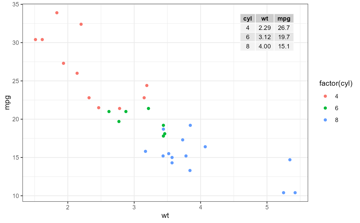
# using defaults
ggplot(mtcars, aes(wt, mpg, colour = factor(cyl))) +
geom_point() +
geom_table(data = df,
aes(x = x, y = y, label = tb))
 # settings aesthetics to constants
ggplot(mtcars,
aes(wt, mpg, colour = factor(cyl))) +
geom_point() +
geom_table(data = df,
aes(x = x, y = y, label = tb),
color = "red",
fill = "#FFCCCC",
family = "serif", size = 5,
angle = 90, vjust = 0)
# settings aesthetics to constants
ggplot(mtcars,
aes(wt, mpg, colour = factor(cyl))) +
geom_point() +
geom_table(data = df,
aes(x = x, y = y, label = tb),
color = "red",
fill = "#FFCCCC",
family = "serif", size = 5,
angle = 90, vjust = 0)
 # passing a theme constructor as argument
ggplot(mtcars,
aes(wt, mpg, colour = factor(cyl))) +
geom_point() +
geom_table(data = df,
aes(x = x, y = y, label = tb),
table.theme = ttheme_gtstripes) +
theme_classic()
# passing a theme constructor as argument
ggplot(mtcars,
aes(wt, mpg, colour = factor(cyl))) +
geom_point() +
geom_table(data = df,
aes(x = x, y = y, label = tb),
table.theme = ttheme_gtstripes) +
theme_classic()
 # transparency
ggplot(mtcars, aes(wt, mpg, colour = factor(cyl))) +
geom_point() +
geom_table(data = df,
aes(x = x, y = y, label = tb),
alpha = 0.5) +
theme_bw()
# transparency
ggplot(mtcars, aes(wt, mpg, colour = factor(cyl))) +
geom_point() +
geom_table(data = df,
aes(x = x, y = y, label = tb),
alpha = 0.5) +
theme_bw()
 ggplot(mtcars, aes(wt, mpg, colour = factor(cyl))) +
geom_point() +
geom_table(data = df,
aes(x = x, y = y, label = tb),
alpha = 0.5, alpha.target = "table.canvas")
ggplot(mtcars, aes(wt, mpg, colour = factor(cyl))) +
geom_point() +
geom_table(data = df,
aes(x = x, y = y, label = tb),
alpha = 0.5, alpha.target = "table.canvas")
 df2 <- tibble(x = 5.45,
y = c(34, 29, 24),
x1 = c(2.29, 3.12, 4.00),
y1 = c(26.6, 19.7, 15.1),
cyl = c(4, 6, 8),
tb = list(tb[1, 1:3], tb[2, 1:3], tb[3, 1:3]))
# mapped aesthetics
ggplot(mtcars,
aes(wt, mpg, color = factor(cyl))) +
geom_point() +
geom_table(data = df2,
inherit.aes = TRUE,
mapping = aes(x = x, y = y, label = tb))
df2 <- tibble(x = 5.45,
y = c(34, 29, 24),
x1 = c(2.29, 3.12, 4.00),
y1 = c(26.6, 19.7, 15.1),
cyl = c(4, 6, 8),
tb = list(tb[1, 1:3], tb[2, 1:3], tb[3, 1:3]))
# mapped aesthetics
ggplot(mtcars,
aes(wt, mpg, color = factor(cyl))) +
geom_point() +
geom_table(data = df2,
inherit.aes = TRUE,
mapping = aes(x = x, y = y, label = tb))
 ggplot(mtcars,
aes(wt, mpg, color = factor(cyl))) +
geom_point() +
geom_table(data = df2,
inherit.aes = TRUE,
colour.target = "table.rules",
mapping = aes(x = x, y = y, label = tb))
ggplot(mtcars,
aes(wt, mpg, color = factor(cyl))) +
geom_point() +
geom_table(data = df2,
inherit.aes = TRUE,
colour.target = "table.rules",
mapping = aes(x = x, y = y, label = tb))
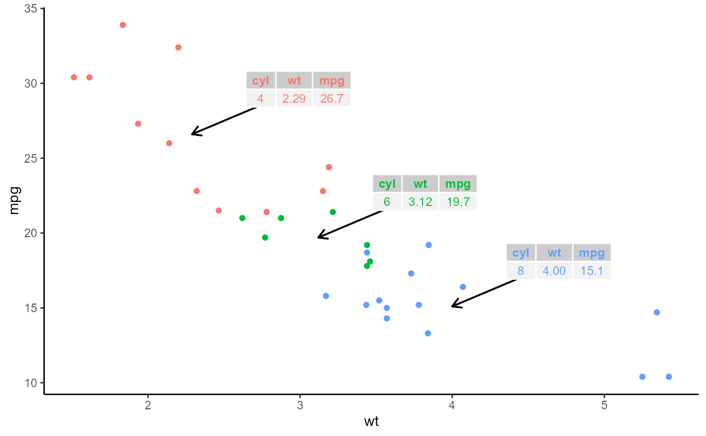
 # nudging and segments
ggplot(mtcars,
aes(wt, mpg, color = factor(cyl))) +
geom_point(show.legend = FALSE) +
geom_table(data = df2,
inherit.aes = TRUE,
mapping = aes(x = x1, y = y1, label = tb),
nudge_x = 0.7, nudge_y = 3,
vjust = 0.5, hjust = 0.5,
arrow = arrow(length = unit(0.5, "lines"))) +
theme_classic()
# nudging and segments
ggplot(mtcars,
aes(wt, mpg, color = factor(cyl))) +
geom_point(show.legend = FALSE) +
geom_table(data = df2,
inherit.aes = TRUE,
mapping = aes(x = x1, y = y1, label = tb),
nudge_x = 0.7, nudge_y = 3,
vjust = 0.5, hjust = 0.5,
arrow = arrow(length = unit(0.5, "lines"))) +
theme_classic()
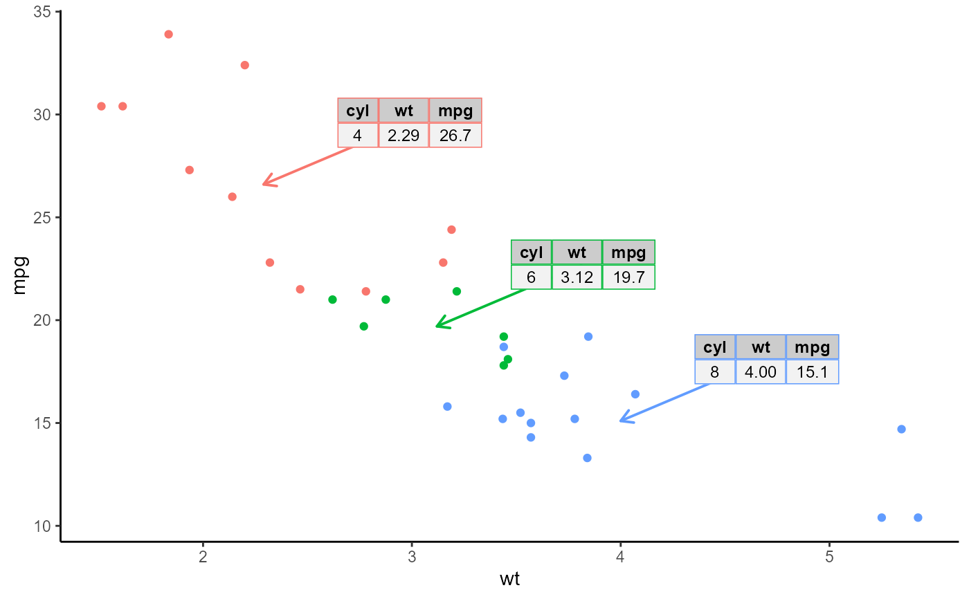
 ggplot(mtcars,
aes(wt, mpg, color = factor(cyl))) +
geom_point(show.legend = FALSE) +
geom_table(data = df2,
inherit.aes = TRUE,
mapping = aes(x = x1, y = y1, label = tb),
nudge_x = 0.7, nudge_y = 3,
vjust = 0.5, hjust = 0.5,
arrow = arrow(length = unit(0.5, "lines")),
colour.target = c("table.rules", "segment")) +
theme_classic()
ggplot(mtcars,
aes(wt, mpg, color = factor(cyl))) +
geom_point(show.legend = FALSE) +
geom_table(data = df2,
inherit.aes = TRUE,
mapping = aes(x = x1, y = y1, label = tb),
nudge_x = 0.7, nudge_y = 3,
vjust = 0.5, hjust = 0.5,
arrow = arrow(length = unit(0.5, "lines")),
colour.target = c("table.rules", "segment")) +
theme_classic()
 # Using native plot coordinates instead of data coordinates
dfnpc <- tibble(x = 0.95, y = 0.95, tb = list(tb))
ggplot(mtcars,
aes(wt, mpg, colour = factor(cyl))) +
geom_point() +
geom_table_npc(data = dfnpc,
aes(npcx = x, npcy = y, label = tb))
# Using native plot coordinates instead of data coordinates
dfnpc <- tibble(x = 0.95, y = 0.95, tb = list(tb))
ggplot(mtcars,
aes(wt, mpg, colour = factor(cyl))) +
geom_point() +
geom_table_npc(data = dfnpc,
aes(npcx = x, npcy = y, label = tb))