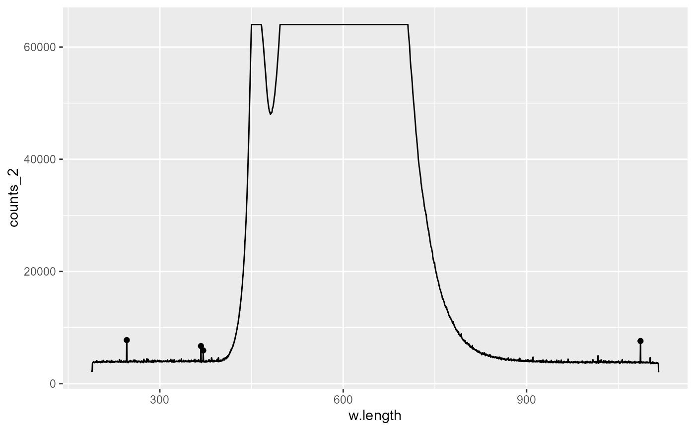
stat_spikes finds at which x positions spikes are located.
Spikes can be either upwards or downwards from the baseline.
Axis flipping is currently not supported.
Usage
stat_spikes(
  mapping = NULL,
  data = NULL,
  geom = "point",
  position = "identity",
  ...,
  height.threshold = 10,
  z.threshold = 9,
  k = 20,
  spike.direction = "both",
  max.spike.width = NA,
  chroma.type = "CMF",
  label.fmt = "%.3g",
  x.label.fmt = label.fmt,
  y.label.fmt = label.fmt,
  x.label.transform = function(x) {
     x
 },
  y.label.transform = function(x) {
     x
 },
  x.colour.transform = x.label.transform,
  na.rm = FALSE,
  show.legend = FALSE,
  inherit.aes = TRUE
)
Arguments
- mapping
The aesthetic mapping, usually constructed with
aesoraes_. Only needs to be set at the layer level if you are overriding the plot defaults.- data
A layer specific dataset - only needed if you want to override the plot defaults.
- geom
The geometric object to use display the data
- position
The position adjustment to use for overlapping points on this layer
- ...
other arguments passed on to
layer. This can include aesthetics whose values you want to set, not map. Seelayerfor more details.- height.threshold
numeric The minimum height of spikes expressed relative to the median amplitude of the baseline local variation of
x.- z.threshold
numeric Modified local \(Z\) values larger than
z.thresholdare detected as boundaries of spikes.- k
integer width of median window used for smoothing; must be odd
- spike.direction
character Controls the direction of spikes to be detected. Accepted arguments are
"up","down","both".- max.spike.width
integer Sets an upper limit to the width in "pixels" of the features detected as spikes.
NA, the default, sets no limit.- chroma.type
character one of "CMF" (color matching function) or "CC" (color coordinates) or a
chroma_spctobject.- label.fmt, x.label.fmt, y.label.fmt
character strings giving a format definition for construction of character strings labels with function
sprintffromxand/oryvalues.- x.label.transform, y.label.transform, x.colour.transform
function Applied to
xoryvalues when constructing the character labels or computing matching colours.- na.rm
a logical value indicating whether NA values should be stripped before the computation proceeds.
- show.legend
logical. Should this layer be included in the legends?
NA, the default, includes if any aesthetics are mapped.FALSEnever includes, andTRUEalways includes.- inherit.aes
If
FALSE, overrides the default aesthetics, rather than combining with them. This is most useful for helper functions that define both data and aesthetics and shouldn't inherit behaviour from the default plot specification, e.g.borders.
Value
A data frame of observations found in the data matching the criterion of being part of a spike. That is to say, the returned data frame not only includes the observation at the tip of the spike but also those on its shoulders.
Details
This stat uses geom_point by default as it is the geom most
likely to work well in almost any situation without need of tweaking. The
default aesthetics set by this stat allow its direct use with
geom_text, geom_label, geom_line, geom_rug,
geom_hline and geom_vline. The formatting of the labels
returned can be controlled by the user.
Note
This stat works nicely together with geoms geom_text_repel and
geom_label_repel from package ggrepel to
solve the problem of overlapping labels
by displacing them. To discard overlapping labels use check_overlap =
TRUE as argument to geom_text.
By default the labels are character values suitable to be plotted as is,
but with a suitable label.fmt argument labels suitable for parsing
by the geoms (e.g., into expressions containing greek letters or super or
subscripts) can be also easily obtained.
Computed variables
- x
x-value at the peak (or valley) as numeric
- y
y-value at the peak (or valley) as numeric
- x.label
x-value of observations in the spike formatted as character
- y.label
y-value of observations in the spike formatted as character
- wl.color
color definition calculated by assuming that x-values are wavelengths expressed in nanometres.
- BW.color
color definition that is either "black" or "white", to ensure high contrast to
wl.color.
Default aesthetics
Set by the statistic and available to geoms.
- label
stat(x.label)
- xintercept
stat(x)
- yintercept
stat(y)
- fill
stat(wl.color)
Required aesthetics
Required by the statistic and need to be set with aes().
- x
numeric, wavelength in nanometres
- y
numeric, a spectral quantity
Spike detection
Spikes are detected based on a modified \(Z\) score calculated from the differenced spectrum. The \(Z\) threshold used should be adjusted to the characteristics of the input and desired sensitivity. The lower the threshold the more stringent the test becomes, with shorter spikes being detected.
The algorithms assume a consistent step size for the underlying
independent variable, e.g., wavelength or time, and should not be applied
if the data do not fulfil this assumption, at least approximately. As
find_spkikes() operates on a single vector, checking this remains
the responsibility of calling functions or methods such as
spikes() and despike().
The algorithm uses running differences to detect abrupt changes in value, compared to an estimate of the baseline variation of the differences, approximating a baseline \(Z\) from MAD and a baseline value from the median differences. Currently, a single estimate of MAD is used but running medians, when possible, as baseline. This comparison detects running differences that are unusually large, in most cases signalling a transition between values near the baseline and far from it, in both directions.
Transitions into- and out of spikes are distinguished based on the median of the non-differenced values, as a descriptor of the data baseline. As for the median of the differences, a running median is used when possible.
This function thus detects the start and end of each spike, and distinguishes upward and downward spikes.
k is the width in number of observations of the window used for
running median smoothing to extract the baseline. A value several times the
width of the broader spike but narrow enough to track broader peaks needs
to be manually set in most cases.
With na.rm = TRUE, NA values are omitted before searching for
spikes and set to 0L in the returned vector.
If all spikes are guaranteed to be one observation-wide and either going up
or down from the baseline, it is possible to detect them based purely on
the z.threshold by passing height.threshold = NA and either
spike.direction = "up" or spike.direction = "down", which
ensures very fast computation.
Parameters of the algorithm need to be adjusted depending on the data, so
inspection of returned values is needed together with adjustment by trial
and error of suitable values for z.threshold,
height.threshold, and k.
The argument to parameter max.spike.width is used in a final stage
to discard spikes detected by the algorithms described above but considered
to be too wide (as a run of successive observations, i.e., detector pixels
in the case of array spectrometers).
See also
find_spikes, which is used internally.
Other stats functions:
stat_color(),
stat_find_qtys(),
stat_find_wls(),
stat_label_peaks(),
stat_peaks(),
stat_wb_box(),
stat_wb_column(),
stat_wb_contribution(),
stat_wb_hbar(),
stat_wb_irrad(),
stat_wb_label(),
stat_wb_mean(),
stat_wb_relative(),
stat_wb_sirrad(),
stat_wb_total(),
stat_wl_strip(),
stat_wl_summary()
Examples
# ggplot() methods for spectral objects set a default mapping for x and y.
# two spurious(?) spikes
ggplot(sun.spct) +
stat_spikes(colour = "red") +
geom_line()
 # no spikes detected
ggplot(sun.spct) +
stat_spikes(colour = "red", z.threshold = 12) +
geom_line()
# no spikes detected
ggplot(sun.spct) +
stat_spikes(colour = "red", z.threshold = 12) +
geom_line()
 # small noise spikes detected
ggplot(white_led.raw_spct) +
stat_spikes(colour = "red") +
geom_line()
# small noise spikes detected
ggplot(white_led.raw_spct) +
stat_spikes(colour = "red") +
geom_line()
 ggplot(white_led.raw_spct) +
stat_spikes(colour = "red") +
stat_spikes(geom = "text", colour = "red", check_overlap = TRUE,
vjust = -0.5, label.fmt = "%3.0f nm") +
geom_line()
ggplot(white_led.raw_spct) +
stat_spikes(colour = "red") +
stat_spikes(geom = "text", colour = "red", check_overlap = TRUE,
vjust = -0.5, label.fmt = "%3.0f nm") +
geom_line()
 # noisy data
ggplot(white_led.raw_spct, aes(w.length, counts_2)) +
stat_spikes(colour = "red",
z.threshold = 10) +
geom_line()
# noisy data
ggplot(white_led.raw_spct, aes(w.length, counts_2)) +
stat_spikes(colour = "red",
z.threshold = 10) +
geom_line()
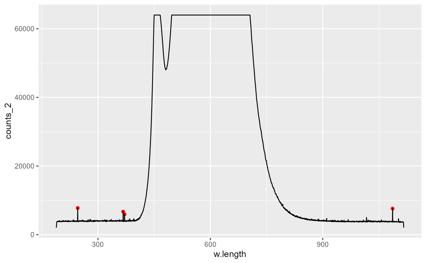
 # with height.threshold to ignore minor spikes
ggplot(white_led.raw_spct, aes(w.length, counts_2)) +
stat_spikes(colour = "red", height.threshold = 15, z.threshold = 10) +
geom_line()
# with height.threshold to ignore minor spikes
ggplot(white_led.raw_spct, aes(w.length, counts_2)) +
stat_spikes(colour = "red", height.threshold = 15, z.threshold = 10) +
geom_line()
 # colour from wavelengths (here black for UV and NIR)
ggplot(white_led.raw_spct, aes(w.length, counts_2)) +
stat_spikes(mapping = aes(colour = after_stat(wl.color)),
height.threshold = 15, z.threshold = 10) +
geom_line() +
scale_colour_identity()
# colour from wavelengths (here black for UV and NIR)
ggplot(white_led.raw_spct, aes(w.length, counts_2)) +
stat_spikes(mapping = aes(colour = after_stat(wl.color)),
height.threshold = 15, z.threshold = 10) +
geom_line() +
scale_colour_identity()