Peaks, Valleys and Spikes
‘ggspectra’ 0.4.0
Pedro J. Aphalo
2026-03-18
Source:vignettes/articles/peaks-and-valleys.Rmd
peaks-and-valleys.RmdIntroduction
This article is only available as part of the on-line documentation of R package ‘ggspectra’. It is not installed in the local computer as part of the package.
Package ‘ggspectra’ extends ‘ggplot2’ with stats, geoms, scales and
annotations suitable for light- or radiation-related spectra. It also
defines ggplot() and autoplot() methods
specialized for the classes defined in package ‘photobiology’ for
storing different types of spectral data. The ggplot()
methods, statistics, and scales in User
Guide: 1 Grammar of Graphics and the autoplot()
methods are described separately in vignette User
Guide: 2 Autoplot Methods.
The new elements can be freely combined with methods and functions defined in packages ‘ggplot2’, ‘scales’, ‘ggrepel’, ‘gganimate’ and other extensions to ‘ggplot2’. This article, focuses on highlighting and annotating peaks, valleys and spikes in plots of spectral data created with R package ‘ggspectra’.
Set up
## Loading required package: SunCalcMeeus## Documentation at https://docs.r4photobiology.info/## Registered S3 methods overwritten by 'ggpp':
## method from
## heightDetails.titleGrob ggplot2
## widthDetails.titleGrob ggplot2##
## Attaching package: 'ggpp'## The following object is masked from 'package:ggplot2':
##
## annotateIntroduction: Peaks, Valleys and Spikes
In a spectrum, maxima of the spectral quantity are called peaks, and minima are called valleys. Spikes are very narrow peaks or valleys. Spikes are frequently caused by detector noise or ambient radiation, such as cosmic rays inpinging on an individual sensing element in a detector array. Anomalous detector elements, usually called hot, cold or dead pixels, can also create spikes. Although spikes are in many cases a “nuisance”, this is not always the case,
When measuring radiation spectra the monochromator acquires data at specific wavelengths, while the true position of peaks may fall in-between the centre of the bands “seen” by the spectrometer. When the optical wavelength resolution and detector pitch of the spectrometer are higher than the accuracy with which the wavelength at the peaks needs to be determined, we can simply search for the wavelengths matching maxima or minima in the acquired data. In this case, the approach is to search for global or local maxima so as to find them in the data. An example of this is when the optical resolution of the monochromator is much lower than the wavelength resolution of the detector array. In an array spectrometer it is a rather frequent case to have a detector array with a wavelength resolution given by the pixel pitch that is significantly better than the wavelength resolution of the grating used as monochromator.
When the accuracy needed is more, the approach used is to fit a curve describing the shape of the peak, and analytically or numerically determine the maxima of the fitted function. This not only requires additional computations but also the choice of a function form capable of describing well the shape of the peak or valley. In this case we first search for peaks, and subsequently fit a function to each of the peaks found, and find the wavelength value at which the derivative of the fitted function is equal to zero. The accuracy of the estimated wavelength at the peak and the height of the peaks are not necessarily both good, one can be better than the other, so it is important to visually check the quality of these estimates. The choice of function to fit depends on the shape of the peaks and the with of the peak compared to the wavelength resolution at which the data have been measured. There are different mathematical formulations in common use. If the wavelength resolution is high compared to the width of the peaks and the data are not affected by noise, using a spline function can be a useful alternative.
In many cases, some peaks are considered “relevant” while others lack interest. Peaks that are much shorter than the tallest ones or peaks that are not locally prominent, are frequently considered irrelevance. When “filtering-out” those local maxima that are of no interest, both creiteria can be combined. In both cases it is possible to set size thresholds that are relative to the data range or fixed and expressed in the same units as the data.
The algorithms used to find, fit and filter valleys is the same as for peaks, but applied to the data after a change of sign. Thus, the explanation above about peaks also applies to valleys.
Spikes are in many cases not of interest and are simply removed from the data. In other cases, spikes may identify defective pixels in an array spectrometer. Very rarely spikes are of interest in themselves, but some cases exist. For example when peaks of interest are narrow compared to the wavelength resolution used for acquiring the spectrum, they may appear in the acquired data as spikes.
In ‘ggspectra’, peaks, valleys and spikes are treated similarly. They are searched for and fitted with functions from package ‘photobiology’. Other related features are wavelengths at specific levels of the spectral response and the “half maximum full width” (HMFW) of peaks. Below most examples are for peaks, and only a few for valleys and spikes to highlight the similarities and differences.
Peaks and Valleys
The formal parameters of functions stat_peaks() and
stat_labels() can be grouped into those controlling the
detection of peaks and valleys: span, strict,
global.threshold, and local.threshold, those
related to fitting of peaks: refine.wl and
method, those affecting the values generated as labels and
colours used to depict the peaks and valleys in plots:
chroma.type, label.fmt,
x.label.fmt, and y.label.fmt, and finally
those related to the use transformations in axis scales:
x.label.transform, y.label.transform, and
x.colour.transform.
Search window: Span
We save a base plot to use in examples.
Using default arguments for the statistic and passing two arguments indirectly to the geometry, creates a plot with many peaks highlighted by small red points.
p0 +
  stat_peaks(colour = "red", size = 1)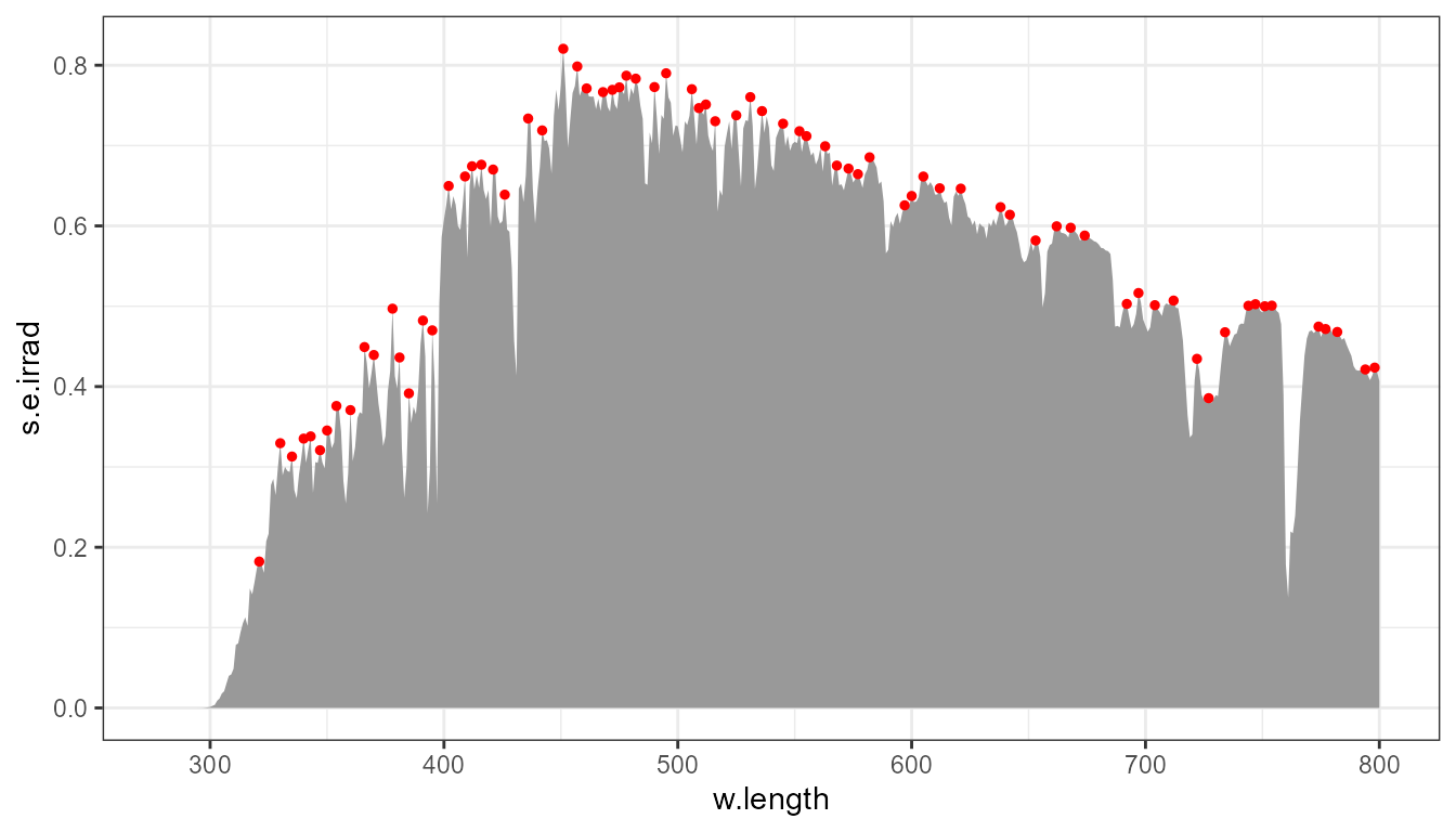
With the argument to parameter span, with default
span = 5, peaks are searched as maxima within a moving
window of width five. Passing an odd integer value sets the
width of window to be used. Passing span = NULL sets the
window width to the whole data set, forcing a search for maximum of the
spectrum as a whole.
p0 +
  stat_peaks(span = NULL, colour = "red", size = 1)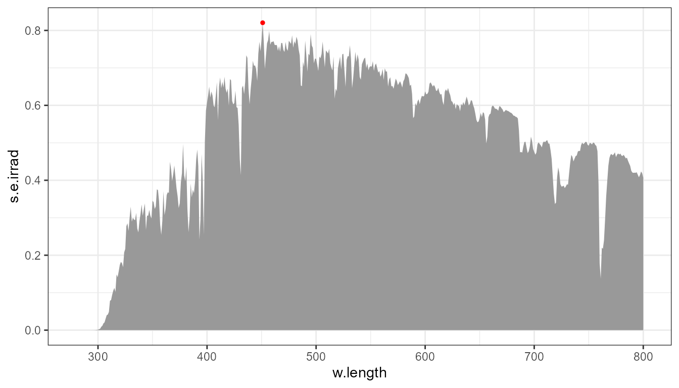
How near to each other are the detected peaks depends on the width of
the moving window, given by the argument passed to span.
This span is given as a number of successive data points along the
x axis, not in wavelength units!
p0 +
  stat_peaks(span = 11, colour = "red", size = 1)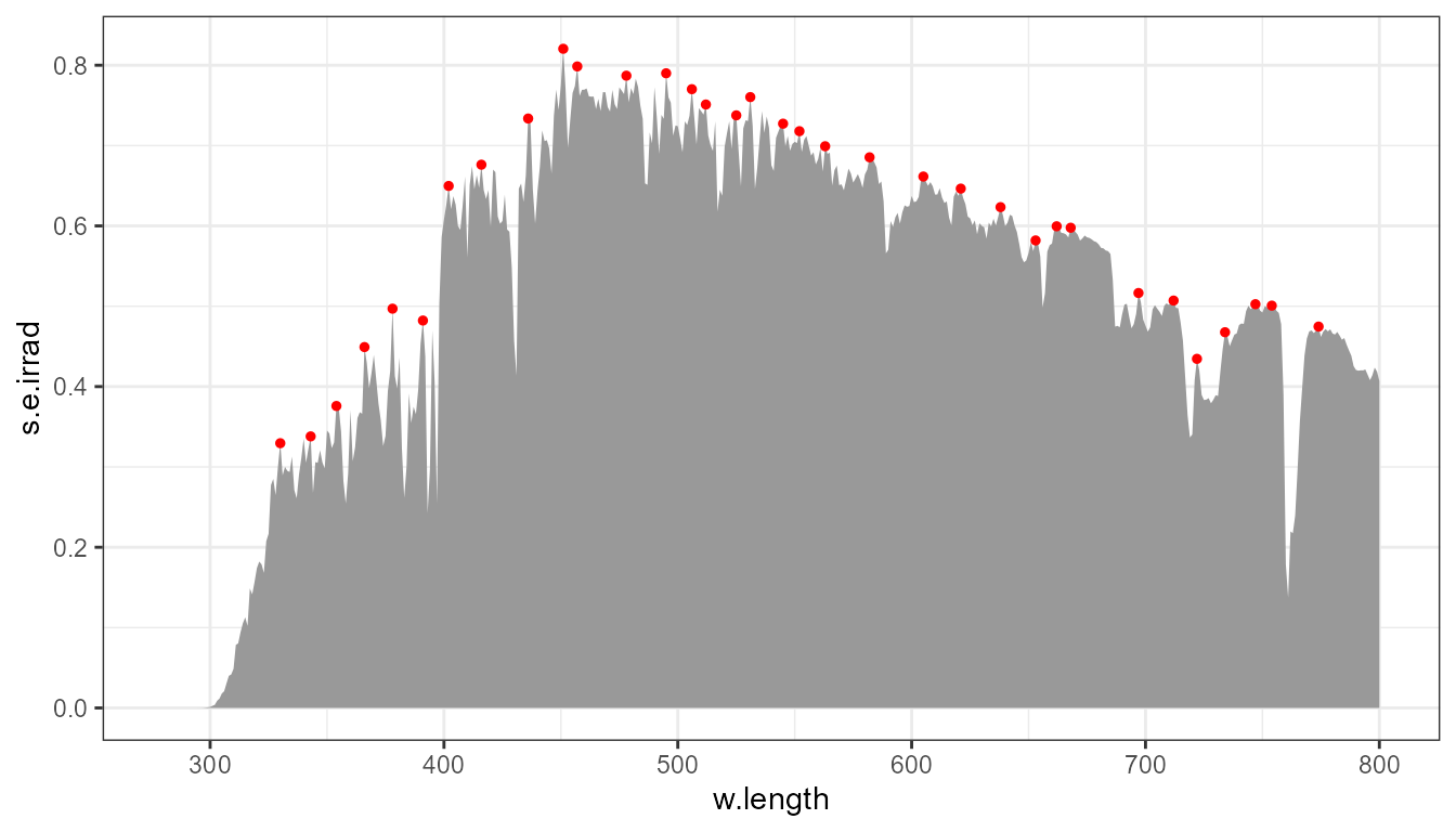
Peak height: global.threshold
Above, the default value for global.threshold is
0.01 and enables the “filtering-out” of the smallest
“peaks”. Passing global.threshold = NULL disables
filtering.
p0 +
  stat_peaks(span = 11, colour = "red", size = 1, global.threshold = NULL)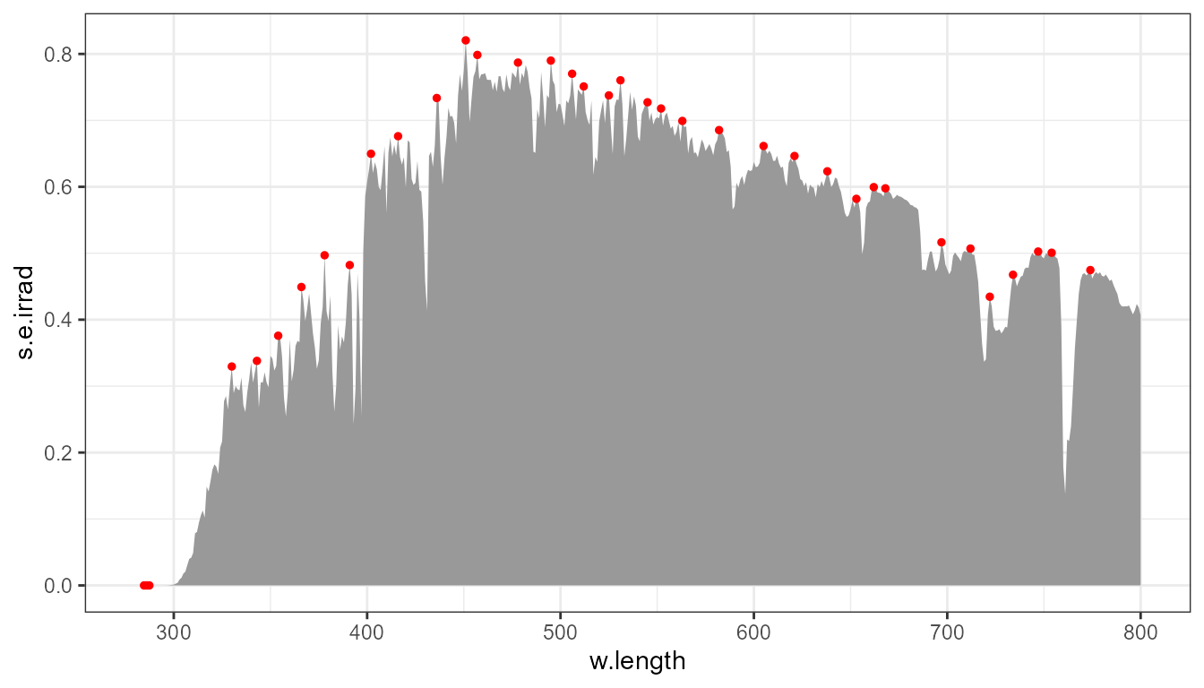
The search for peaks can be constrained by giving a minimum height
threshold in data units. For example, we can keep only peaks exceeding a
value of 0.7 for s.e.irrad, the variable mapped to the
y aesthetic. We indicate the use of data units by enclosing the
argument for global.threshold in a call to
I(). (Function I() sets the class of its
argument to "AsIs", thus such values can be saved in
variables and passed as arguments also by name.)
p0 +
  stat_peaks(global.threshold = I(0.7), colour = "red", size = 1)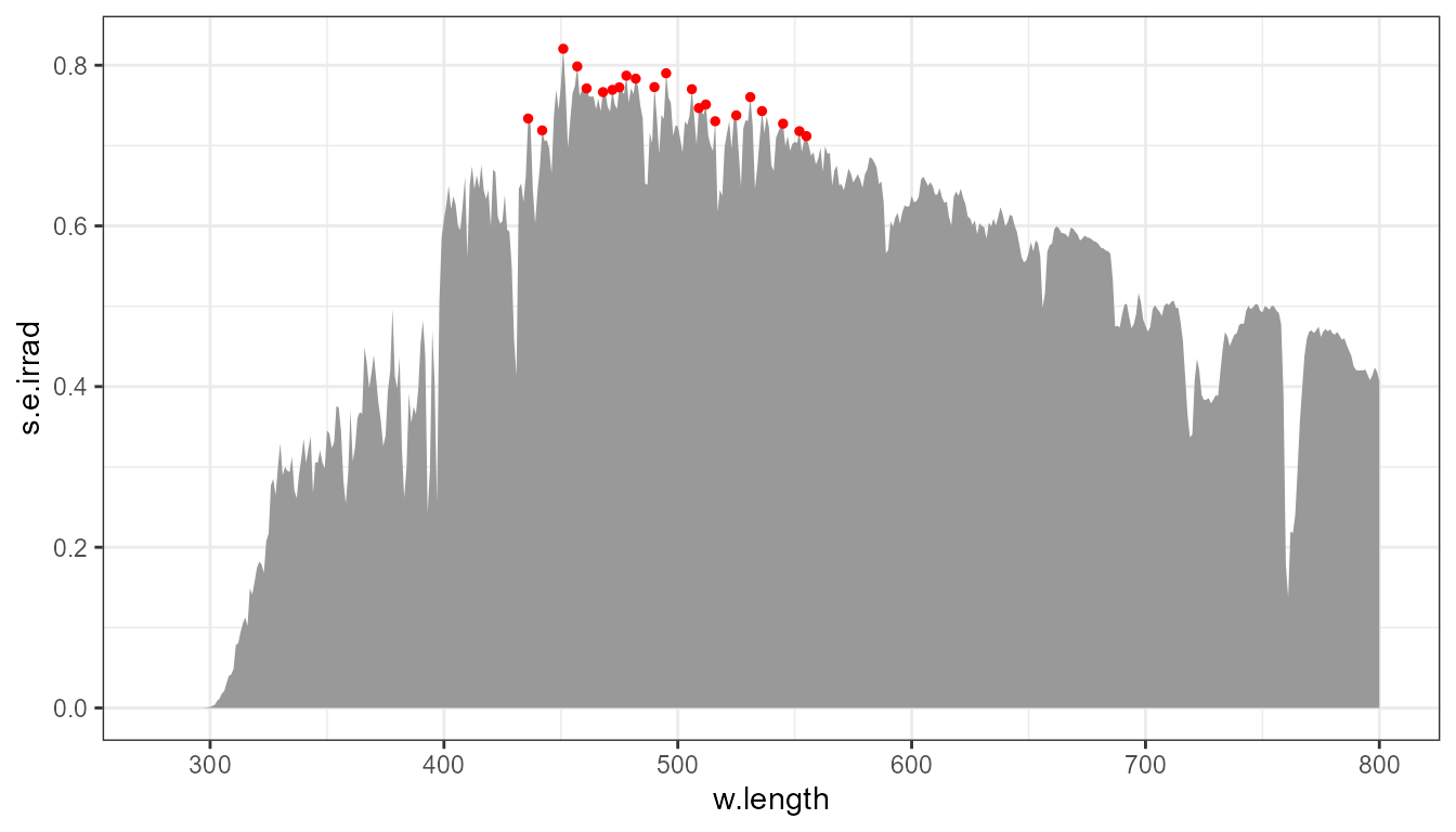
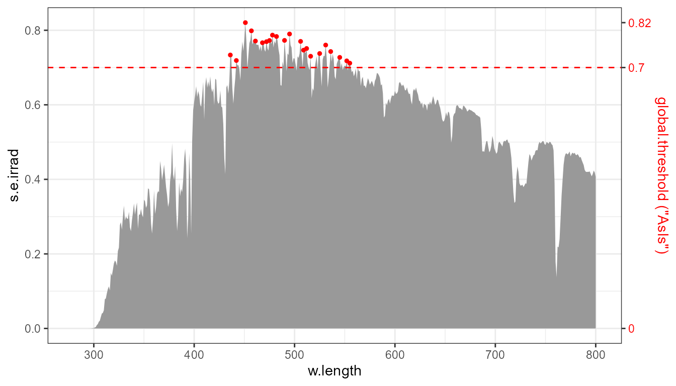
The same plot as above, annotated with the threshold and the range of the observations.
To limit the detected (and highlighted) peaks to taller ones than by default, we can limit the search, for example, to the top 1/3 of the y range, by filtering-out those in the lower 2/3 of the y range of the data.
p0 +
stat_peaks(global.threshold = 2/3, colour = "red", size = 1) 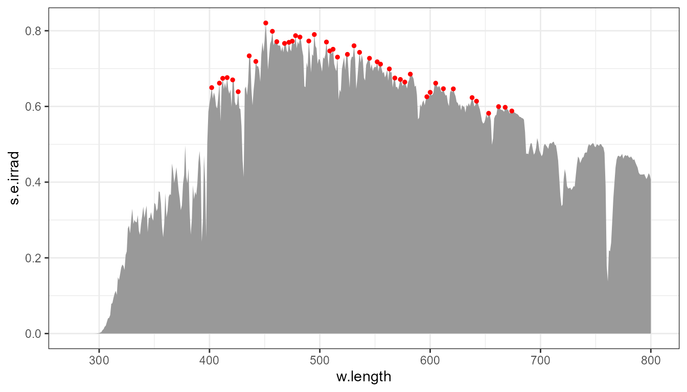
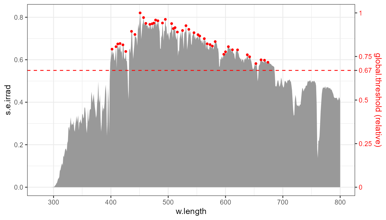
The same plot annotated to show how the threshold range of 0\ldots 1 relates to the data range.
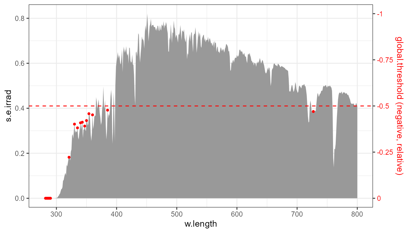
Very rarely the tallest peaks need to be discarded, but if needed
this can be achieved by passing a number in -1\ldots 0 as argument to
global.threshold.
p0 +
  stat_peaks(global.threshold = -0.5, colour = "red", size = 1)
The same plot as above, annotated.
Global thresholds work similarly with stat_valleys(),
and numbers closer to one apply a more stringent threshold than smaller
values.
p0 +
  stat_valleys(global.threshold = 0.5, colour = "blue", size = 1)
And the same plot as above, annotated with the threshold used and the possible range.

Peak prominence: local.threshold
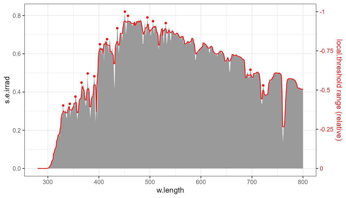
A different criterion for “filtering-out” peaks is their prominence compared to their neighbours. As implemented here, it is based on comparing the peak height to the lowest data value within the same window where the peak is found. In this example, only peaks whose height compared to the smallest value in their window differs by at least 1/10 of the data range are kept.
p0 +
  stat_peaks(colour = "red", size = 1, span = 11, local.threshold = 0.03)
The same plot as above, annotated with the running median, used as local reference for the threshold.
By default the reference for the local prominence of a peak is the
median observation within the window. Alternatively, the farthest value
in the window can be used as reference, in which case larger
local.threshold values tend to be needed to obtain a
similar effect with "farthest" as with
"median". The reference used is controlled by parameter
local.reference.
p0 +
  stat_peaks(colour = "red", size = 1, span = 11,
             local.reference = "farthest", local.threshold = 0.1)
The same plot as above, annotated with the running minimum line.

As for global.threshold we can specify the minimum local
height in data units with a call to I().
p0 +
  stat_peaks(colour = "red", size = 1, span = 11, local.threshold = I(0.03))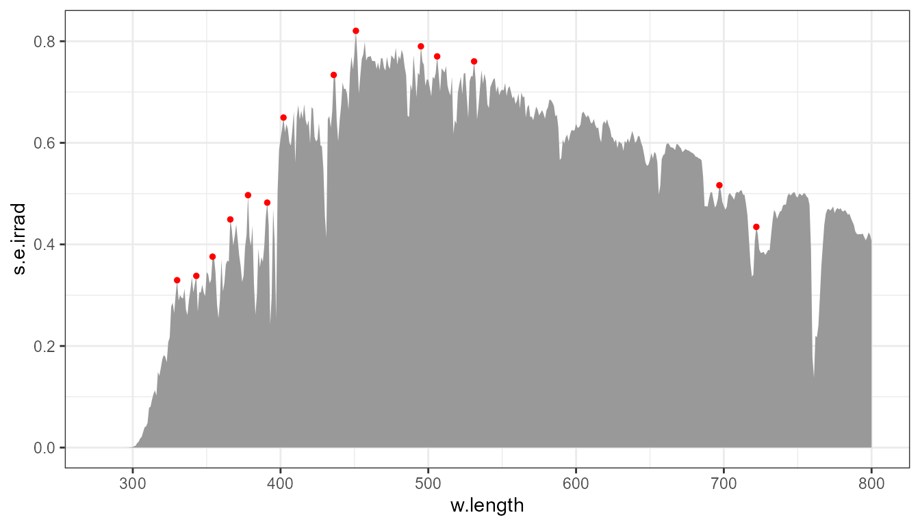
It is important to keep in mind that span,
local.threshold and global.threshold can be
combined. However, span modifies the effect of
local.threshold by widening the window in which the median
or farthest value is searched.
p0 +
  stat_peaks(colour = "red", size = 1,
             span = 5,
             local.threshold = I(0.01),
             global.threshold = I(0.5))
Local thresholds also are implemented in stat_valleys()
or work similarly as in stat_peaks(). The reference lines
are as for peaks but the distance is assessed downwards from the line
instead of upwards, even if arguments passed to
local.threshold are in 0\ldots
1 or data units as for peaks.
Fitting peaks: refine.wl
The solar spectrum data used above has values at 522 different
wavelengths and a difference between successive wavelength values of
\approx 1 \,\mathrm{nm}. Above we used
the default geom_point(). To demonstrate the effect of
fitting, we use geom_text().
p0 +
  stat_peaks(span = NULL,
             colour = "red", size = 3, geom = "text", vjust = -0.5,
             x.label.fmt = "%#.5g nm")
p0 +
  stat_peaks(span = NULL, refine.wl = TRUE,
             colour = "red", size = 3, geom = "text", vjust = -0.5,
             x.label.fmt = "%#.5g nm")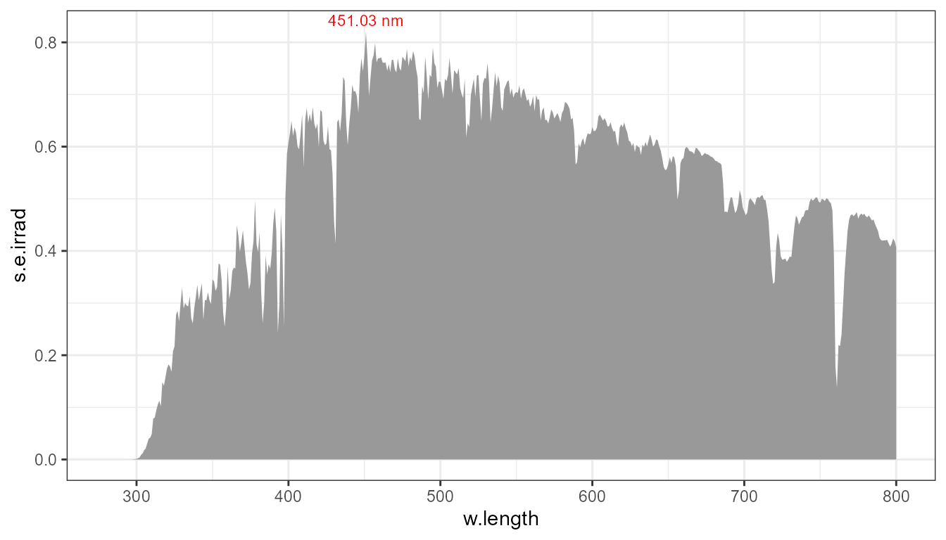
Labels: label.fmt, x.label.fmt,
y.label.fmt, and chroma.type
Above, x.label.fmt was used without explanation.
Statistics stat_peaks() and stat_valleys() not
only return the rows in plot data corresponding to peaks or
valleys but in addition add columns with computed RGB colour definition
values matching the visual colour at the peak’s wavelength and
character strings for both x (wavelength) and
y (spectral quantity) values at the peaks.
The default chroma.type = "CMF" rarely needs to be
overriden. Above, colour = "red", size = 3, vjust = -0.5
are all arguments passed to geom_text unchanged.
p0 +
  stat_peaks(span = NULL, refine.wl = TRUE, geom = "text")
As the returned values are colour definitions, for them to display
correctly scale_fill_identity() and
scale_colour_identity() must be added to the plot when
using them.
p0 +
  stat_peaks(span = NULL, refine.wl = TRUE,
             geom = "label", colour = "white", vjust = "bottom") +
  expand_limits(y = 0.85) +
  scale_fill_identity()
The formatting of labels frequently needs to the set by users. Format
strings are as described for R function sprintf() and are
described in detail in its help page. The format is a
character string with a place holder for the numeric value
of x or y at the peak. While the default
label.fmt = "%.3g" gives a bare number with three
significant digits both for x and y as below, above we
used x.label.fmt = "%#.5g nm" indicating a number with five
significant digits followed by a literal " nm". The use of
# ensures that trailing zeros are displayed.
Labels are not only generated for wavelengths but also for the
spectral quantity. The argument to parameter label.fmt is
used for both for both variables, unless overriden by arguments topassed
to x.label.fmt and/or y.label.fmt. The
y label variable needs to be mapped to be used as the
x label is be default mapped to the label
aesthetic. The format defines a character string that after
substitution of the place holder needs to be parsed into an R
expression. This makes it possible to include plotmath
expressions.
p0 +
  stat_peaks(mapping = aes(label = after_stat(y.label)),
             span = NULL, refine.wl = TRUE,
             y.label.fmt = "%.3f~W~m^{-2}~nm^{-1}", parse = TRUE,
             geom = "label", colour = "white", vjust = "bottom") +
  expand_limits(y = 0.85) +
  scale_fill_identity()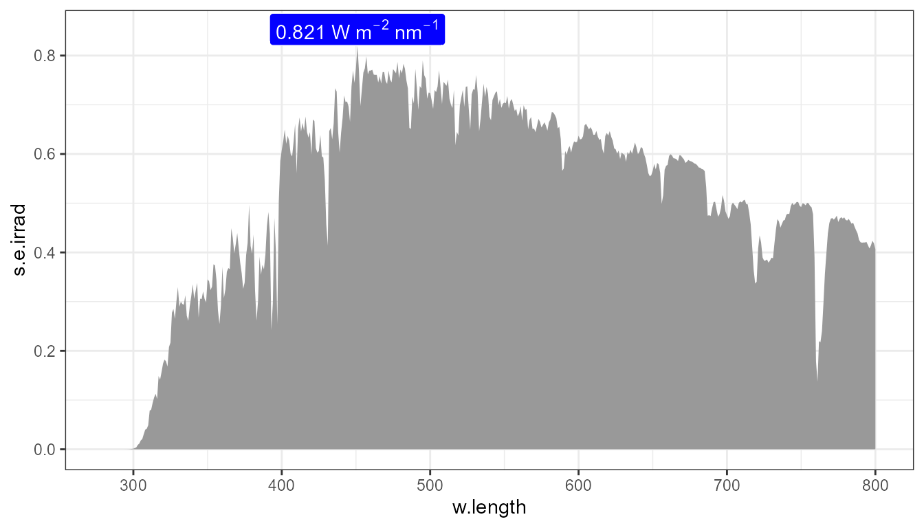
There are different possible ways of combining x and y labels. Here is an example relying on the statistic to format the labels.
p0 +
  stat_peaks(mapping =
               aes(label = paste(after_stat(y.label),
                                "\" at \"",
                                after_stat(x.label),
                                sep = "*"),
                   color = after_stat(BW.colour)), # precomputed contrasting colour
             span = NULL, refine.wl = TRUE,
             x.label.fmt = "%.4g~nm",
             y.label.fmt = "%.3f~W~m^{-2}~nm^{-1}",
             parse = TRUE,
             geom = "label",
             vjust = "bottom", size = 3) +
  expand_limits(y = 0.85) +
  scale_fill_identity() +
  scale_color_identity()
The formatting can also be done within the call to aes()
as below just using the numeric values of X and y.
(This approach is general and can be used with any ggplot statistic that
returns numeric values.)
p0 +
  stat_peaks(mapping =
               aes(label = sprintf("%.3f~W~m^{-2}~nm^{-1}*\" at \"*%.4g~nm",
                                   after_stat(y), after_stat(x))),
             span = NULL, refine.wl = TRUE,
             parse = TRUE,
             geom = "label", colour = "white", vjust = "bottom", size = 3) +
  expand_limits(y = 0.85) +
  scale_fill_identity()
The colours used above for fill are computed from the
wavelength with method color_of() from package
‘photobiology’, using the default colour matching function
("CMF") for human vision.
Values at half maximum
In the case of light spectra with a single peak, we may be interested
in highlighting the wavelengths at half maximum, or at some other value
of the spectral quantity. This is implemented in
stat_find_wls(). The algorithm used is extremely simple, if
no y value in the data falls exactly at the
target, the x value at the target is estimated by
linear interpolation between the two bordering observations. The formal
parameters related to colour and labels are identical to those in
stat_peaks() and stat_valleys(). The only new
parameter is target that makes it possible to set the
target y values in different ways. The default is to use half
the height of the tallest peak in the curve.
my.format <- "%#.1f nm"

ggplot(white_led.source_spct) +
  geom_spct() +
  stat_find_wls() +
  stat_find_wls(aes(colour = after_stat(BW.colour)),
                x.label.fmt = my.format,
                geom = "label", hjust = c(1.1, -0.1)) +
  expand_limits(y = 0.7) +
  scale_colour_identity() +
  scale_fill_identity()
In the case of a long pass filter, we may be interested in showing the wavelengths at 10% and 50% transmittance (\tau_\lambda = 0.1 and \tau_\lambda = 0.5).
my.format <- "%#.1f nm"

ggplot(yellow_gel.spct) +
  geom_spct() +
  stat_find_wls(target = c(0.1, 0.5)) +
  stat_find_wls(target = c(0.1, 0.5), geom = "text", hjust = 1.2)
Values at wavelength
The value of the spectral quantity at a user specified wavelengths
can be shown with stat_find_qts() that similarly to
stat_find_wls() uses interpolation as needed.
my.format <- "%#.1f nm"

ggplot(yellow_gel.spct) +
  geom_spct() +
  stat_find_qtys(target = 500) +
  stat_find_qtys(target = 500, geom = "text", hjust = 1.2)
Spikes
Function stat_spikes() is very similar in its interface
to stat_peaks() and stat_valleys(). However,
as the algorithm used is different, the parameters used to control the
search for spikes are different, while those related to the formatting
of labels and colours are identical.
A more suitable example spectrum than sun.spct is one
with very narrow peaks as some discharge lamps, like a low pressure
mercury fluorescent tube. However, the data set used here has been
reduced in size by decreasing the wavelength resolution in featureless
regions. Because of this, a warning is triggered although in this case
three spikes are anyway found after passing suitable arguments.
library(photobiologyLamps)

p1 <-
  ggplot(lamps.mspct$Eiko.F36T8.BLB) +
  geom_spct() +
  geom_point(size = 1)
In the first plot all observations are shown as points.
p1
p1 + stat_spikes(z.threshold = 30, max.spike.width = 5,
                 size = 1, colour = "red")
## 'compute_group()' assumes consistent w.length steps! max step / min step = 3.6
With different arguments a lower z threshold and higher maximum width, we detect more spikes. Whether the large peak should be considered a spike or not is debatable. In addition, because of the uneven wavelength steps, the shoulder of the large peak is wrongly detected as being part of a spike.
p1 +
  stat_spikes(z.threshold = 20, max.spike.width = 10,
              size = 1, colour = "red")
## 'compute_group()' assumes consistent w.length steps! max step / min step = 3.6
Complete plot examples
In the bare-bones examples above most statistics and their features were exemplified individually. Plots as used in real-life situations in many cases a much more elaborated. The examples in the present section combine different features into finished plots such as those that could be used in a presentation or publication.
In these examples additional “building blocks” provided by packages ‘ggspectra’ and ‘ggplot2’ are used in addition to those specific to annotation of peaks, valleys and spikes.
Wavelengths at target y values
my.format <- "%.1f nm"

ggplot(normalise(yellow_gel.spct)) +
  geom_spct(colour = "black", linewidth = 0.35) +
  stat_find_wls(target = c(0.1, 0.5, 0.9), colour = "red") +
  stat_find_wls(target = c(0.1, 0.5, 0.9), geom = "rug", colour = "red") +
  stat_find_wls(aes(colour = after_stat(BW.colour)),
                target = c(0.1, 0.5, 0.9),
                x.label.fmt = my.format,
                geom = "label", size = 3, hjust = 1.1) +
  scale_colour_identity() +
  scale_fill_identity() +
  scale_y_Tfr_continuous(breaks = c(0, 0.10, 0.50, 0.90, 1.00),
                         Tfr.type = "internal") +
  scale_x_wl_continuous() +
  theme_classic()
Peaks and valleys in one plot
The plot below makes use of the different features described above.
In this plot each of stat_peaks() and
stat_valleys() are used to add two leyers, using two
different geometries, geom_point() and
geom_label(). To demonstrate its effect,
local.threshold = 0.15 is passed only when using
geom_label() so that only prominent peaks and valleys are
labelled with the fitted wavelengths. The wavelengths are correct only
to the 1\,\mathrm{nm} resolution of the
sampling used for the extraterrestrial solar spectrum data used as input
for the simulations.
my.format <- "%.3g nm" # used twice, easier to set here

ggplot(sun.spct) +
  geom_line() +
  stat_peaks(span = 31, geom = "point", colour = "red", refine.wl = TRUE) +
  stat_peaks(mapping = aes(fill = after_stat(wl.colour),
                           color = after_stat(BW.colour)),
             span = 31, local.threshold = 0.045,
             label.fmt = my.format,
             refine.wl = TRUE,
             geom = "label", size = 3, hjust = -0.1, angle = 90) +
  stat_valleys(span = 31, refine.wl = TRUE,
               geom = "point", colour = "blue") +
  stat_valleys(mapping = aes(fill = after_stat(wl.colour),
                             color = after_stat(BW.colour)),
               span = 31, local.threshold = 0.1,
               label.fmt = my.format,
               refine.wl = TRUE,
               geom = "label", size = 3, hjust = 1.1, angle = 90) +
  expand_limits(y = c(-0.05, 1)) + # make room for label
  scale_fill_identity() +
  scale_color_identity() +
  scale_x_wl_continuous() +
  scale_y_s.e.irrad_continuous()
The colours used above for fill are computed from the
wavelength of each peak.
Exploring the data returned by statistics
With geom_debug_group() from package ‘gginnards’ we can
explore the data data frame passed by the statistic to the
geometry. geom_debug_group() by default prints the value
returned by head() as a tibble without adding a layer to
the plot. Thus, its behaviour is atypical.
library(gginnards)

ggplot(sun.spct) +
  geom_spct() +
  stat_peaks(span = 31,
             geom = "debug_group",
             dbgfun.data = "head",
             dbgfun.data.args = list(n = 20))
## [1] "PANEL 1; group(s) -1; 'draw_function()' input 'data' (head):"
## x y PANEL group x.label y.label wl.colour BW.colour label fill
## 1 378 0.4969714 1 -1 378 0.497 #000000 white 378 #F8766D
## 2 416 0.6761818 1 -1 416 0.676 #1600D9 white 416 #00B9E3
## 3 451 0.8204633 1 -1 451 0.82 #0400FF white 451 #00C19F
## 4 478 0.7869773 1 -1 478 0.787 #0041DD white 478 #D39200
## 5 495 0.7899872 1 -1 495 0.79 #008A45 white 495 #93AA00
## 6 531 0.7603297 1 -1 531 0.76 #00FF00 black 531 #00BA38
## 7 582 0.6853736 1 -1 582 0.685 #FFAE00 black 582 #FF61C3
## 8 605 0.6614323 1 -1 605 0.661 #FF1300 white 605 #DB72FB
## 9 662 0.5995383 1 -1 662 0.6 #660000 white 662 #619CFF
## 10 747 0.5025733 1 -1 747 0.503 #000000 white 747 #F8766D
## 11 774 0.4746771 1 -1 774 0.475 #000000 white 774 #F8766D
## xintercept yintercept
## 1 378 0.4969714
## 2 416 0.6761818
## 3 451 0.8204633
## 4 478 0.7869773
## 5 495 0.7899872
## 6 531 0.7603297
## 7 582 0.6853736
## 8 605 0.6614323
## 9 662 0.5995383
## 10 747 0.5025733
## 11 774 0.4746771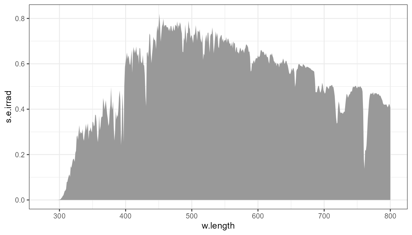
This approach can be also used to explore the effect of passing different arguments in the call to the stattistic.
ggplot(sun.spct) +
  geom_spct() +
  stat_peaks(mapping = aes(label = after_stat(y.label)),
             span = NULL, refine.wl = TRUE,
             y.label.fmt = "%.3f~W~m^{-2}~nm^{-1}",
             colour = "white", vjust = "bottom",
             geom = "debug_group",
             dbgfun.data = "head") +
  expand_limits(y = 0.85) +
  scale_fill_identity()
## [1] "PANEL 1; group(s) -1; 'draw_function()' input 'data' (head):"
## x y PANEL group x.label y.label wl.colour
## 1 451.0269 0.8205136 1 -1 451 0.821~W~m^{-2}~nm^{-1} #0400FF
## BW.colour label fill xintercept yintercept vjust colour
## 1 white 0.821~W~m^{-2}~nm^{-1} #0400FF 451.0269 0.8205136 bottom white