User Guide: 2 Autoplot Methods
‘ggspectra’ 0.4.0
Pedro J. Aphalo
2026-03-18
Source:vignettes/userguide2-autoplot-methods.Rmd
userguide2-autoplot-methods.RmdIntroduction
Package ggspectra extends ggplot2 with
stats, geoms and annotations suitable for light and radiation spectra.
It also defines ggplot() and autoplot()
methods specialized for the classes defined in package
photobiology for storing different types of spectral data.
This vignette describes the use of these autoplot()
methods.
The package uses ‘ggplot2’, ‘photobiology’ and ‘photobiologyWavebands’. More importantly it defines specializations of methods defined in ‘ggplot2’ and exports methods specialized for classes defined in package ‘photobiology’, consequently both ‘ggplot2’ and ‘photobiology’ are loaded and attached automatically when package ‘ggspectra’ is loaded. (When using earlier versions earlier than 0.9.26 these packages had to be loaded and attached explicitly.)
## Loading required package: photobiology## Loading required package: SunCalcMeeus## Documentation at https://docs.r4photobiology.info/
library(ggspectra)
library(ggrepel)

# ensure all labels are plotted
options(ggrepel.max.overlaps = Inf)
We will use an individual sunlight spectrum sun.spct and
a short time series of spectra sun_evening.spct and
`sun_evening.mspct’, from ‘photobiology’ for examples.
summary(sun.spct)## Summary of source_spct [522 x 3] object: sun.spct
## Wavelength range 280-800 nm, step 0.9230769-1 nm
## Label: sunlight, simulated
## Measured on 2010-06-22 09:51:00 UTC
## Measured at 60.20911 N, 24.96474 E; Kumpula, Helsinki, FI
## Variables:
## w.length: Wavelength [nm]
## s.e.irrad: Spectral energy irradiance [W m-2 nm-1]
## s.q.irrad: Spectral photon irradiance [mol s-1 m-2 nm-1]
## --
## w.length s.e.irrad s.q.irrad
## Min. :280.0 Min. :0.0000 Min. :0.000e+00
## 1st Qu.:409.2 1st Qu.:0.4115 1st Qu.:1.980e-06
## Median :539.5 Median :0.5799 Median :2.929e-06
## Mean :539.5 Mean :0.5160 Mean :2.407e-06
## 3rd Qu.:669.8 3rd Qu.:0.6664 3rd Qu.:3.155e-06
## Max. :800.0 Max. :0.8205 Max. :3.375e-06
summary(sun_evening.spct)## Summary of source_spct [7,965 x 3] object: sun_evening.spct
## containing 5 spectra in long form
## Wavelength range 290-1000 nm, step 0.34-0.47 nm
## Label: cosine.hour.9
## time.01 measured on 2023-06-12 18:38:00.379657 UTC
## time.02 measured on 2023-06-12 18:39:00.797266 UTC
## time.03 measured on 2023-06-12 18:40:00.714554 UTC
## time.04 measured on 2023-06-12 18:41:00.768459 UTC
## time.05 measured on 2023-06-12 18:42:00.769065 UTC
## Measured at 60.227 N, 24.018 E; Viikki, Helsinki, FI
## Variables:
## w.length: Wavelength [nm]
## s.e.irrad: Spectral energy irradiance [W m-2 nm-1]
## --
## w.length s.e.irrad spct.idx
## Min. : 290.0 Min. :0.00000 time.01:1593
## 1st Qu.: 474.4 1st Qu.:0.02315 time.02:1593
## Median : 654.8 Median :0.03892 time.03:1593
## Mean : 651.6 Mean :0.03659 time.04:1593
## 3rd Qu.: 830.3 3rd Qu.:0.04888 time.05:1593
## Max. :1000.0 Max. :0.07503
summary(sun_evening.mspct)## Summary of source_mspct [5 x 1] object: sun_evening.mspct
## # A tibble: 5 × 8
## spct.idx class dim w.length.min w.length.max colnames multiple.wl time.unit
## <chr> <chr> <chr> <dbl> <dbl> <list> <dbl> <Duratio>
## 1 time.01 sourc… [1,5… 290 1000. <chr> 1 1s
## 2 time.02 sourc… [1,5… 290 1000. <chr> 1 1s
## 3 time.03 sourc… [1,5… 290 1000. <chr> 1 1s
## 4 time.04 sourc… [1,5… 290 1000. <chr> 1 1s
## 5 time.05 sourc… [1,5… 290 1000. <chr> 1 1sWe change the default theme for ggplots.
Using the autoplot() methods
The most automatic way of plotting spectral data stored in one of the
classes defined in package photobiology is to use the
autoplot() methods (for compatibility with versions <
0.9.25 plot() remains as a deprecated name for the same
methods). As autoplot() methods defined by ‘ggplot2’ they
take advantage of all the data and metadata stored in objects of the
special classes used to store spectra. This allows the automatic
construction of axis labels as quantities and units are well
defined.
The basics
Here we use the same example source_spct object from
package ‘photobiology’ to demonstrate parameters common to all
autoplot() methods for spectra. Methods for plotting of
objects of most classes defined in package ‘photobiology’ are available.
Function spct_classes() lists these classes.
# the classes
spct_classes()
## [1] "calibration_spct" "raw_spct" "cps_spct" "filter_spct"
## [5] "reflector_spct" "source_spct" "object_spct" "response_spct"
## [9] "chroma_spct" "solute_spct" "generic_spct"## [1] "autoplot.calibration_spct" "autoplot.cps_spct"
## [3] "autoplot.filter_spct" "autoplot.generic_spct"
## [5] "autoplot.object_spct" "autoplot.raw_spct"
## [7] "autoplot.reflector_spct" "autoplot.response_spct"
## [9] "autoplot.source_spct"The simplest possible call to autoplot() needs only one
argument, the object to plot.
autoplot(sun.spct)
In contrast to the examples in the User Guide 1, here we
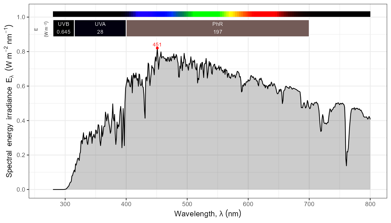
obtain directly an annotated plot of the solar spectrum at ground level.
This would be of limited use without the possibility to adjust the
design and components of the ggplot object created. One
approach is to use the grammar of graphics to add to the plot. However,
it is also possible to control many features of the plot by passing
additional arguments in the call to autoplot().
User-provided arguments override the defaults.
When plotting source_spct and response_spct
objects we can change the basis of expression of spectral irradiance and
spectral response from "energy" to "photon".
Be aware that by design, within one plot all spectral values and derived
summaries will always use the same base of expression.
autoplot(sun.spct, unit.out = "photon")
We can build and area ("spct") plot instead the default
line plot.
autoplot(sun.spct, geom = "spct")
We can build and area + line (c("spct", "line")) plot
instead the default line plot.
If a single object contains multiple spectra in long form, they are all plotted. In this case no summary values are displayed as they would overlap.
autoplot(sun_evening.spct)
We can rename the factor that identifies the spectra, changing the title of the key for the lines.
autoplot(sun_evening.spct, idfactor = "Time")
In addition to the autoplot() methods for individual
spectra and spectra in stored long form (_spct classes),
there are autoplot() methods available for collections of
spectra (_mspct classes). Collections of spectra like
sun_evening.mspct can be plotted also automatically, as
they are combined on-the-fly and plotted as shown above in the example
for sun_evening.spct. The methods for collections of
spectra and for multiple spectra in long form behave almost identically.
The parameters are the same as those in the autoplot()
methods for multiple spectra in long form described above.
We use in the next examples a simple collection of five spectra.
These are the same five spectra as above
(sun_evening.spct), but stored in an object of a different
class. The plotting of objects of all the classes for collections of
spectra defined in package ‘photobiology’ is similar. Function
mspct_classes() lists all the classes for collections of
spectra defined in package ‘photobiology’.
# the classes
mspct_classes()
## [1] "calibration_mspct" "raw_mspct" "cps_mspct"
## [4] "filter_mspct" "reflector_mspct" "source_mspct"
## [7] "object_mspct" "solute_mspct" "response_mspct"
## [10] "chroma_mspct" "generic_mspct"## [1] "autoplot.calibration_mspct" "autoplot.cps_mspct"
## [3] "autoplot.filter_mspct" "autoplot.generic_mspct"
## [5] "autoplot.object_mspct" "autoplot.raw_mspct"
## [7] "autoplot.reflector_mspct" "autoplot.response_mspct"
## [9] "autoplot.source_mspct"The plot using defaults is identical to that above.
autoplot(sun_evening.mspct)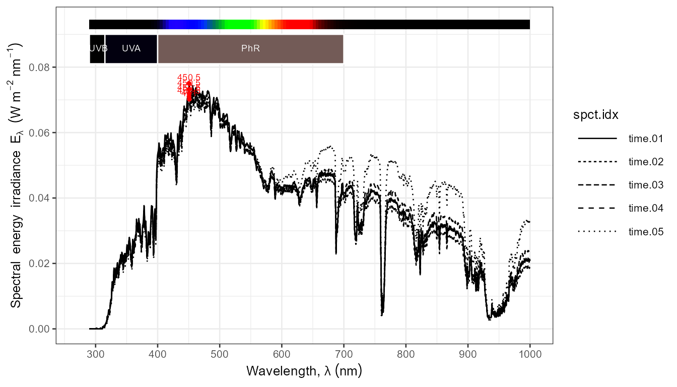
We can choose a different name for the factor identifying the spectra in the collection.
autoplot(sun_evening.mspct, idfactor = "Time")
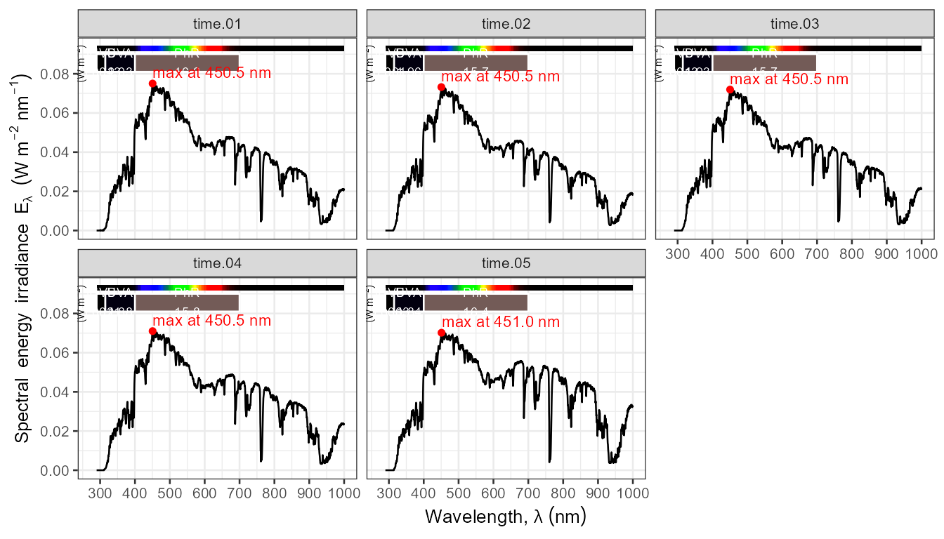
With facets, there is only one spectrum per panel. Summaries per waveband are shown.
autoplot(sun_evening.spct, facets = TRUE)
Above we showed the default faceting by passing
facets = TRUE. We can set the number of columns by passing
a number. For panels in one column we pass facets = 1, and
for two columns we pass facets = 2, and so on.
autoplot(sun_evening.mspct, facets = 2)
autoplot(sun_evening.mspct, geom = "spct", facets = 2)
Contrary to "gg" objects created with package ‘ggplot2’,
the data embedded in the "gg" objects created with these
autoplot() methods retains the attributes used by package
‘photobiology’, including the class.
## Summary of source_spct [522 x 2] object: anonymous
## Wavelength range 280-800 nm, step 0.9230769-1 nm
## Label:  sunlight, simulated
## Measured on  2010-06-22 09:51:00  UTC
## Measured at 60.20911 N, 24.96474 E; Kumpula, Helsinki, FI
## Variables:
##  w.length: Wavelength [nm]
##  s.e.irrad: Spectral energy irradiance [W m-2 nm-1]
## --
##     w.length       s.e.irrad
##  Min.   :280.0   Min.   :0.0000
##  1st Qu.:409.2   1st Qu.:0.4115
##  Median :539.5   Median :0.5799
##  Mean   :539.5   Mean   :0.5160
##  3rd Qu.:669.8   3rd Qu.:0.6664
##  Max.   :800.0   Max.   :0.8205
This makes it possible to trace the origin of the data, and also to apply specialised methods to them.
Note: When using ‘ggplot2’ (>= 4.0.0)
@ can be used instead of $ to extract
components like data data, and should be preferred for new
scripts.
Wavelengths
We can zoom into the spectrum, by providing a wavelength range in
nanometres. Here we pass a vector of two numbers as argument, but any
object for which a range() method is available can also be
used, including longer numeric vectors, objects of one the spectrum
classes, such as class source_spct, or a
waveband definition. In the case of vectors of length two,
NA can be used to signal the use of the default limit.

The range can be also expanded in a similar way, for example to ensure consistent limits across plots of spectra of different wavelength ranges.
We can show summaries for different wavebands, by passing them to
parameter w.band. We can pass either individual wavebands
or lists of wavebands. First a list of wavebands created with a
constructor, here showing the limits based on the ISO standard.

A single waveband can also be created with a generic constructor.

NULL as argument for w.band is replaced by
a waveband covering the full range of the spectral data. The whole
range is the range plotted, which is controlled by the argument
passed to range.
autoplot(sun.spct, w.band = NULL)
Summarizing the examples above, arguments passed to
range and w.band play very different roles.
Parameter range, gives the wavelengths to include in the
plot, and the default for range is always the range of
wavelengths in the spectrum being plotted. The argument to
w.band is only used for the annotations and
decorations, described in a later section in more detail.
The effect of range is different to the effect of
ggplot2::xlim() as range is used to
trim (\approx subset) the
spectral data before passing it to ggplot,
using interpolation when needed (see
photobiology::trim_wl()). In contrast xlim
changes the limits of the scale, and discards data for all wavelengths
not within the range (equivalent to action of
photobiology::clip_wl()). The difference is subtle when the
spectrum has high wavelength resolution but can result in
inconsistencies among plots.
The default argument to parameter w.band can be changed
by setting the R option "photobiology.plot.bands" to a
single waveband object or to a list waveband objects.
Function set_w.band_default() allows to set this option
using the same syntax as described for parameter w.band.
See package ‘photobiologyWavebands’ for waveband constructors for ISO
and other waveband definitions in common use, and package ‘photobiology’
for defining your own.
set_w.band_default(w.band = Plant_bands())Normalization
How already normalized spectral data are plotted by these
autoplot() methods has changed during the history of the
package. Currently, the normalization can be selected by passing an
argument to norm as explained in this section.
We first consider the case of spectral data that has not been
previously normalized. These data are by default plotted as is,
except for the possible conversion into a different quantity or base of
expression. If the argument passed to norm is one of
"max" or "min" or a numeric value for a
wavelength in nanometres, the normalization is applied after the unit or
quantity conversion and the data subsequently plotted. If the argument
passed to norm is one of "skip",
"update" (the default) or "undo" the spectral
data are plotted as is.
We next consider the case of spectral data that has not been
previously normalized. If the argument passed to norm is
one of "max" or "min" or a numeric value for a
wavelength in nanometres, the normalization is applied after the unit or
quantity conversion and the data subsequently plotted. In other words,
the previous normalization is replaced by the new one. If the argument
passed to norm is one of "skip" or
"update" (the default) a new normalization is applied after
the unit or quantity conversion reusing the criterion previsouly used to
normalize the data passed as argument to "data". The
difference between "skip" and "update" is that
the former issues a warning if an update is needed and the later does
not. If the argument passed to norm is "undo"
the existing normalization is reverted if possible before
plotting. Whether “undoing” a normalization is possible depends on full
metadata stored in the object attributes, a feature implemented in
‘photobiology’ (>= 0.14.0).
autoplot(sun.spct, geom = "spct", norm = "max")## Normalization 'norm = max' applied before plotting."
Normalization is reflected in the y-scale tick labels and
axis title. In addition, summaries by waveband are no longer expressed
as irradiances but instead as a contribution to the total, i.e., the
area under the curve. To emphasize this geom = "spct" is
used instead of the default.
“Parallel” summaries
All plotting of multiple spectra shown above were done with the
default plot.data = "as.is". We can also plot a row-wise
summary (wavelength by wavelength, or parallel summaries) of
the spectra in the collection, here the mean of the
spectra. Currently implemented only for spectra with identical
wavelength vectors and of the same class. Of the different supported
functions, "mean" and "median" are likely the
most useful.
autoplot(sun_evening.mspct, plot.data = "mean")
Summary quantities by waveband
Although the defaults result in the addition of frequently useful
annotations, the autoplot() methods accepts arguments for
several parameters that make possible flexible control of the
annotations. Currently, numerical summaries can be added automatically
to plots only when a single spectrum is plotted per plot panel.
In this first example we pass "mean" as argument to
label.qty, to print means instead of integrals in the
labels. Note that the units and quantity labels for the waveband
summaries have also changed.
autoplot(sun.spct, label.qty = "mean")
Two label.qty values need explanation. The first one,
"relative" displays in labels the relative contribution of
the integral of each waveband, to the sum of the integrals of all
wavebands displayed in the plot. The second one,
"contribution" displays in labels the integral of each
waveband divided by the integral of the whole spectrum displayed in the
plot. Consequently, this second option should be interpreted with
caution, as the spectral data is unlikely in many cases to include the
whole emission or absorption spectrum of a source. Adding
.pc to the arguments, that is, using
"relative.pc" or "contribution.pc", results in
the corresponding values being displayed as percentages.
When using "contribution.pc" unless the summarized
wavebands cover the whole range of wavelengths in the spectrum, the sum
of the summary values is less than 100%.
autoplot(sun.spct, label.qty = "contribution.pc") When using
 "relative.pc" the sum adds to 100.
autoplot(sun.spct, label.qty = "relative.pc")
Automatic annotations
Which annotations are included can be controlled through
parameter annotations. It accepts a character
vector, or a list of character vectors as argument. Three
values have special meaning if at the head of the vector (with index =
1): "=" means override the current defaults with the
annotations that follow in the vector, "+" means add to the
current default the annotations that follow, and "-" means
remove from the current default the annotations that follow. A
NULL value means use package-defined defaults as is,
"" means no annotations, and "reserve.space"
means no annotations, but expand axis limits and set identity scales
ready for manually adding annotations. Used together with
"-", "title*", "peaks*" and
"valleys*" are wildcards that remove all flavours
of each of these annotations. In cases when the intention is to both add
and remove annotations from the default, the argument to parameter
annotations can be a list of character vectors, which are
interpreted as above but operated upon sequentially.
Which annotations are included by default can be changed by setting R
option "photobiology.plot.annotations" to a character
vector with the names of the desired default annotations. Function
set_annotations_default() allows to set or modify this
option using the same syntax as described for parameter
annotations.
| annotation | default for classes | overrides |
|---|---|---|
| “boxes” | all | “segments” |
| “segments” | none | “boxes” |
| “color.guide” | all | |
| “peaks” | all | “peak.labels” |
| “peak.labels” | none | “peaks” |
| “valleys” | none | “valley.labels” |
| “valley.labels” | none | “valleys” |
| “wls” | none | “wls.labels” |
| “wls.labels” | none | “wls” |
| “labels” | all | |
| “summaries” |
source_spct, response_spct,
filter_spct, reflector_spct
|
|
| “boundaries” | raw_spct |
|
| “title” | none | |
| “title:type” | none | |
| “title:type:type” | none | |
| “title:type:type:type” | none |
Titles come in different flavours. Package ‘ggplot2’ supports titles,
subtitles and captions. The "title" as argument to
parameter annotation of autoplot() methods and
of function autotitle() takes up to three optional
modifiers separated by colons that can be used to specify the contents
of the automatic title, subtitle and caption. Currently
supported modifiers are shown in the table below. If the metadata item
is not stored in the spectral object, the title or subtitle will show
NA. See the documentation of packages ‘photobiology’ and
‘ooacquire’ for information on how to set and unset attributes of
spectral objects. To add an arbitrary title and/or subtitle to a plot,
use either function ggtitle() or function
labs() from package ‘ggplot2’.
| Modifier | text source used |
|---|---|
objt |
name of the object plotted |
class |
class of the plotted object |
what |
what.measured attribute |
when |
when.measured attribute |
where |
where.measured attribute |
how |
how.measured attribute |
inst.name |
spectrometer name |
inst.sn |
spectrometer serial number |
comment |
comment attribute |
none |
no title, no subtitle or no caption |
For example "title:objt", the default for
"title", adds a title with the name of the object being
plotted. what, when, where and
how use the what.measured,
when.measured, where.measured and
how.measured attributes if available. For example
"title:what:when" will use the what.measured
attribute for the title and the when.measured attribute for
the subtitle.
We add a title, subtitle and caption.

We use “none” as a filler so that only subtitle and caption are added to the plot.

With "boundaries", we add one or two horizontal dashed
lines showing the valid range of values. It does not override any other
annotation. (The boundary line is shown in red when a plot displays
out-of-range spectral data.)

We can list all the annotations to be included in a plot, in which
case "=" is optional so as to maintain compatibility with
earlier versions.
autoplot(sun.spct,
     annotations = c("=", "labels", "summaries", "color.guide", "peaks", "boundaries"))
As indicated in the table above, some annotations override other
annotations which fulfil a similar role. Here "segments"
overrides the "boxes", included in the default
annotations.

We can also remove some of the default annotations on a case by case basis.

The behaviour of some annotations can be tweaked. Below we add
"valleys" as annotations, and control with
span how close to each other are the peaks and valleys
found.

The annotations "peak.labels" and
"valley.labels" override "peaks" and
"valleys". They use the repulsive geometry
geom_label_repel from package ‘ggrepel’.
autoplot(sun.spct,
         annotations = list(c("+", "peak.labels"),
                            c("-", "boxes", "summaries", "labels")),
         span = 21)


Passing "" as argument to annotations
results in a plot with no annotations, and no extra expansion of scale
limits.
autoplot(sun.spct, annotations = "")
Passing "reserve.space" as argument to
annotations results in a plot with no annotations, but with
scale limits expanded so as to receive annotations.
autoplot(sun.spct, annotations = "reserve.space")
The size of the font used for the annotations is controlled by
argument text.size.

Argument ylim allows to manually set the limits of the
y axis using the same syntax as in
package ‘ggplot2’. The annotations are still automatically positioned,
and the range extended to make space for them. In other words the values
passed to ylim still give the “space” available for
plotting data.
 The time base of the spectral unit or the duration of the exposure is
stored as metadata. As demonstrated here using spectral data integrated
over 24 h, a one-day-long exposure, the units in the axis labels change
according to the value stored in the metadata.
getTimeUnit(sun.daily.spct)## [1] "day"
autoplot(sun.daily.spct)
Even though the autoplot() methods can return a finished
plot, the returned object is a ggplot object and can be
built upon by adding additional elements like facets,
aesthetics and even additional layers. We pass
idfactor = NA to suppress the mapping of the spectra to
linetype.
autoplot(sun_evening.spct, facets = 2) +
  geom_vline(xintercept = c(400, 700), linetype = "dashed")
It is possible to construct and bind the spectra on-the-fly, and to
use arbitrary variable names for the index factor. This works
automatically as long as row binding is done with function
rbindspct() which saves the name of the factor.
filter_no_yes.spct <-
  rbindspct(list(sun = sun.spct, filtered = yellow_gel.spct * sun.spct),
            idfactor = "Light source")
autoplot(filter_no_yes.spct)
In the examples above the source_spct object
sun.spct was used. The autoplot() methods for
other spectral classes have only slight differences. We show some
examples for filter_spct objects. For a long-pass filter
the wavelength at half maximum is more interesting than peaks or
valleys.
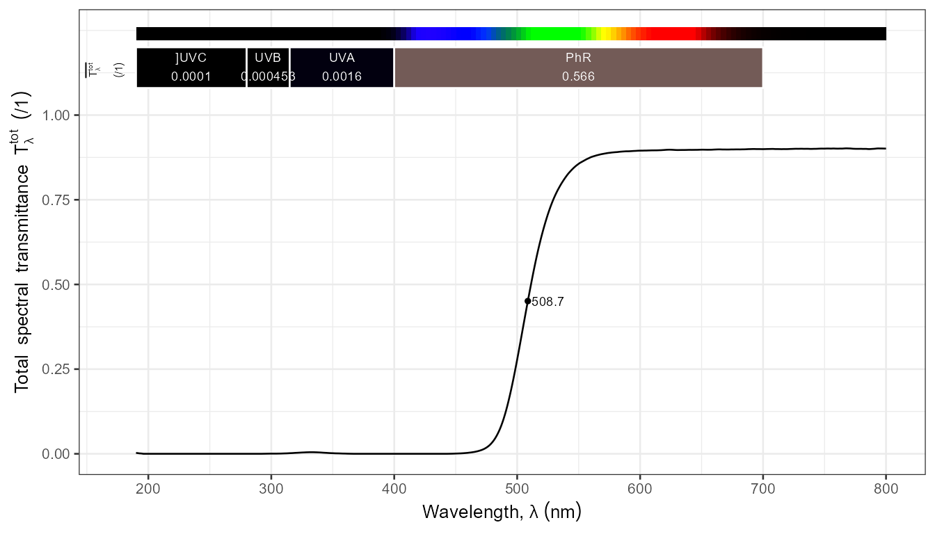
In many cases it is possible to convert on-the-fly the quantity plotted. In this case, given that the data are clipped as absorbance, a fixed target of A = 2 for the cut-off to be labelled with the wavelength is appropriate.
autoplot(yellow_gel.spct, plot.qty = "absorbance", wls.target = 2,
         annotations = list(c("-", "peaks"), c("+", "wls")))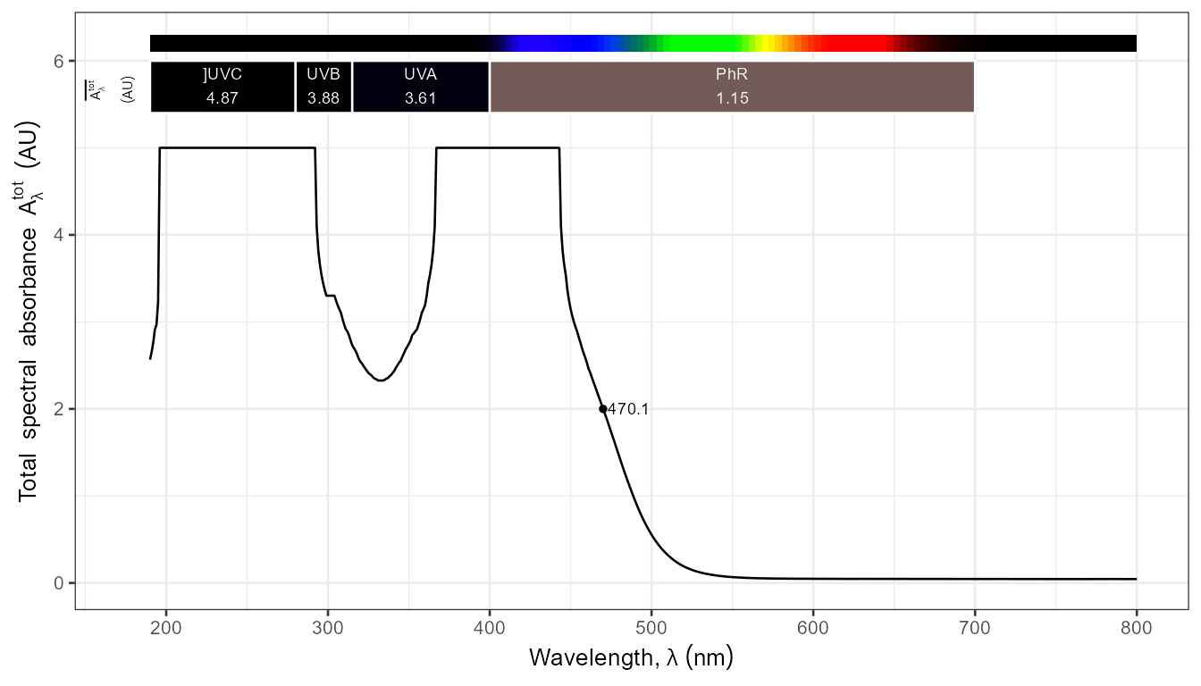
If one needs to, one can add a suitable layer function, geom or stat, using ‘local’ data or add an annotation as shown here.
autoplot(sun.spct,
         w.band = UV_bands("CIE"),
         geom = c("spct", "line"),
         range = c(280, 400),
         unit.out = "photon") +
  geom_vline(xintercept = c(280, 315, 340, 400), linetype = "dotted")
In the case of quantities like transmittance which have a certain range of valid values, both upper and lower boundaries are highlighted, but in other cases only one, or even none depending on the possible valid ranges for the spectral quantities.

Differently from other classes raw_spct and
cps_spct objects can contain multiple columns of data,
normally measured different integration times, and meant to be combined
before conversion into physical quantities. In the case of raw
instrument counts data, if the spectral object contains an instrument
descriptor as metadata, the upper boundary is set to the maximum counts
of the detector.

Both raw_spct and cps_spct objects contain
multiple data columns when integration time bracketing has been used
during data acquisition. In such cases, if one wants to plot only one of
the raw spectra, one can extract the columns as usual in R using the
extraction operator ([ ]). The single remaining column of
spectral data is automatically renamed.
Editing plots and adding layers
Using colors when adding to a plot generated by the
autoplot() methods is more involved than usual, one has to
take into account that the identity scale is in use for color in
annotations, and a ggplot can make use of only one scale for a given
aesthetic. For this same reason no color key in generated
automatically.
autoplot(sun_evening.mspct, annotations = c("-", "peaks")) +
  aes(color = ifelse(spct.idx == "time.05", "black", "darkred")) +
  theme(legend.position = "none")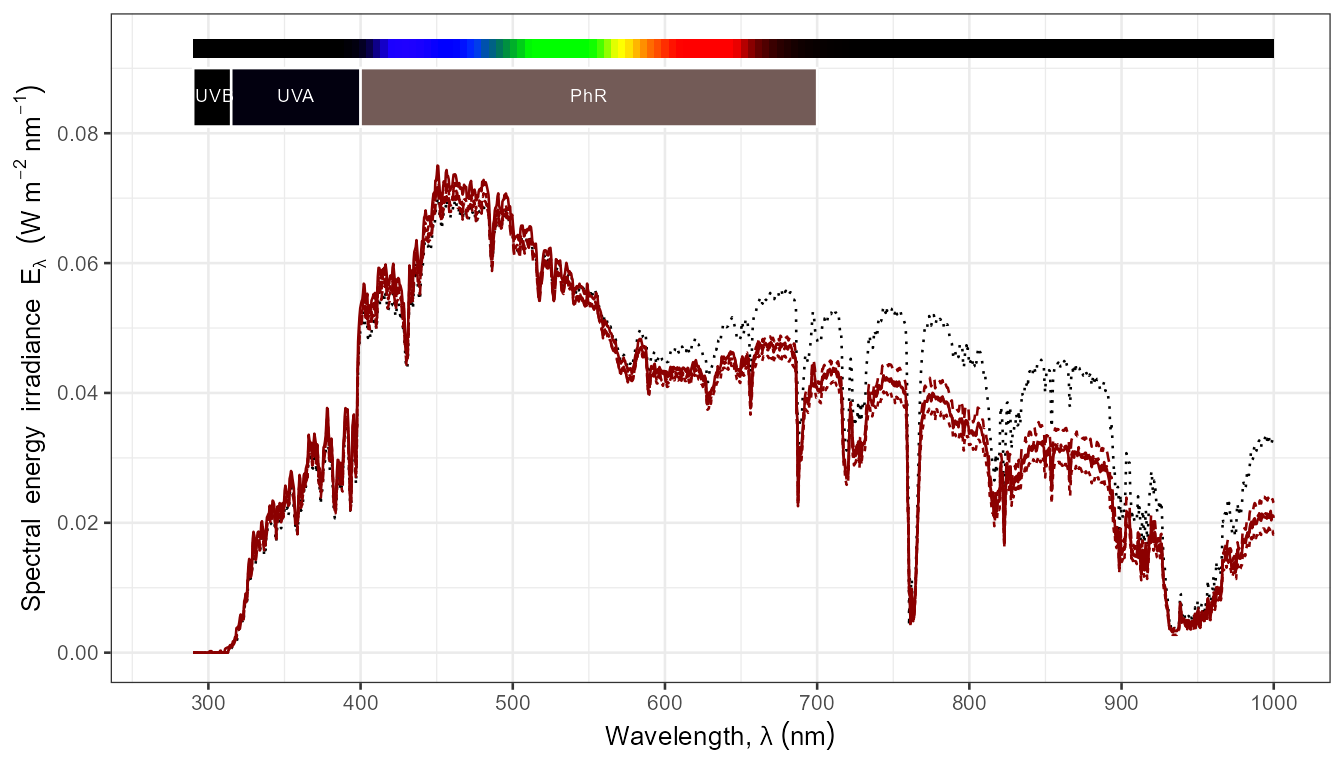
Plots created with autoplot() methods are
ggplot objects and can be customized, bearing in mind that
any added layers will be plotted on top or existing layers (that is
unless we make use of methods from package ‘gginnards’ that allow
insertion of layers at any position in a ggplot
object).
Here we replace the default peaks annotations with a custom one, but still take advantage of other defaults like nice axis labels and other annotations.
autoplot(sun_evening.mspct, annotations = c("-", "peaks"), facets = TRUE) +
  stat_peaks(span = NULL, color = "red") +
  stat_peaks(span = NULL, geom = "text",
             label.fmt = "max at %3.1f nm",
             vjust = -0.5, hjust = 0,
             color = "red", size = 3)