Mixture Models
‘ggpmisc’ 1.0.0.9000
Pedro J. Aphalo
2026-07-08
Source:vignettes/articles/mixture-models.Rmd
mixture-models.RmdAims of ‘ggpmisc’ and caveats
Package ‘ggpmisc’ makes it easier to add to plots created using ‘ggplot2’ annotations based on fitted models and other statistics. It does this by wrapping existing model fit and other functions. The same annotations can be produced by calling the model fit functions, extracting the desired estimates and adding them to plots. There are two advantages in wrapping these functions in an extension to package ‘ggplot2’: 1) we ensure the coupling of graphical elements and the annotations by building all elements of the plot using the same data and a consistent grammar and 2) we make it easier to annotate plots to the casual user of R, already familiar with the grammar of graphics.
To avoid confusion it is good to make clear what may seem obvious to some: if no plot is needed, then there is no reason to use this package. The values shown as annotations are not computed by ‘ggpmisc’ but instead by the usual model-fit and statistical functions from R and R packages. The same is true for model predictions, residuals, etc. that some of the functions in ‘ggpmisc’ display as lines, segments, or other graphical elements.
It is also important to remember that in most cases data analysis including exploratory and other stages should take place before annotated plots for publication are produced. Even though data analysis can benefit from combined numerical and graphical representation of the results, the use I envision for ‘ggpmisc’ is mainly for the production of plots for publication or communication. In case case, whether used for analysis or communication, it is crucial that users cite and refer both to ‘ggpmisc’ and to the underlying R and R packages when publishing plots created with functions and methods from ‘ggpmisc’.
Preliminaries
Other packages are loaded in the section they are used.
Attaching package ‘ggpmisc’ also attaches package ‘ggpp’ as it provides several of the geometries used by default in the statistics described below. Package ‘ggpp’ can be loaded and attached on its own, and has separate documentation.
As we will use text and labels on the plotting area we change the default theme to an uncluttered one.
old_theme <- theme_set(theme_classic())Introduction
Mixture Models are relatives of clustering approaches, and can be applied in different situations. The overall idea is that the observations originate in two or more distinct populations but they are in a mixture, i.e., it is not known which observations belongs to which component (distinct group or population).
Fitting of mixture models aims at estimating the value of the parameters for the individual populations, without classifying the observations. This can be useful in many contexts including fitting of univariate and multivariate theoretical probability distributions like the Normal or Gamma, and also to regression problems.
One obvious case for fitting two components is a population formed by females and males. A different case, with two or three components depending on dominance, is a trait controlled by a single gene measured in an F2 population. Thus, in the case of Normal mixtures, if multiple distinct components are expected, estimates of the mean and standard deviation for each Normal distribution and their standard errors, plus an estimate of the fraction of observations in each group are estimates.
As of ‘ggpmisc’ (>= 0.6.3) the fitting of mixtures of Normal
distributions is supported. Currently the only package supported is
‘mixtools’ and a single method from it normalmixEM().
Fitted models in stat_distrmix_line() and
stat_normal_eq()
Both stat_distrmix_line() and
stat_normal_eq() are designed for flexibility while still
attempting to keep their implementation and use rather straightforward.
As much as possible, from a user’s viewpoint, the interface is similar
to other statistics in ‘ggpmisc’. One key difference is that they their
input from a single aesthetic, x, rather than from two
aesthetics, x and y.
These two statististics also differ from other model fit functions in ‘ggpmisc’ in that the prediction and equations from ungrouped data are grouped according to the fitted components of the mixture. This grouping has one more level than the number of components in the mixture, corresponding to the sum of the components. It is possible to select whether only the components, only the sum of the components or all, components plus their sum, are included in the returned data frame passed to the geometries.
In the current implementation the number of components in the mix,
k, is an input. Other R packages do provide ways of
automating the selection of k but this requires knowledge
on the shape of the individual distributions. The reason is that if
there is a mismatch in shape, an automatic algorithm tends to select too
large a value for k to compensate, as this can increase the
proportion of variation that the fitted model explains. As in the
wrapped fit function, the default is k = 2.
I use for the first example the well known data for Yellowstone’s geiser Faithful on the waiting time between eruptions. Simpler examples are shown in the help page.
The default mapping groups the data for the predicted lines without assigning a visible aesthetic. In these examples, a histogram is plotted in the first layer and the Normal distributions on top of it. By default the fitted model equation is formualted as the sum of the distributions, meanwhile lines for the components and their sums are plotted.
ggplot(faithful, aes(x = waiting)) +
  geom_histogram(aes(y = after_stat(density)), alpha = 0.33, bins = 20) +
  stat_distrmix_line(aes(colour = after_stat(component),
                         fill = after_stat(component)),
                     outline.type = "upper",
                     geom = "area", linewidth = 1, alpha = 0.25,
                     fit.seed = 123) +
  stat_distrmix_eq(aes(colour = after_stat(component)), fit.seed = 123) +
  expand_limits(y = 0.06) # make space for the equation above the histogram
An argument passed to parameter components can be used
to select which components to plot, either "members", their
"sum" or "all", i.e., the members plus their
sum. Below, only the members are plotted and their individual
equations.
ggplot(faithful, aes(x = waiting)) +
  geom_histogram(aes(y = after_stat(density)), alpha = 0.33, bins = 20) +
  stat_distrmix_line(aes(colour = after_stat(component),
                         fill = after_stat(component)),
                     outline.type = "upper",
                     geom = "area", linewidth = 1, alpha = 0.25,
                     components = "members", fit.seed = 123) +
  stat_distrmix_eq(aes(colour = after_stat(component)),
                   components = "members", fit.seed = 123,
                   eq.digits = 3)
Below, only the sum of the members is plotted.
ggplot(faithful, aes(x = waiting)) +
  geom_histogram(aes(y = after_stat(density)), alpha = 0.33, bins = 20) +
  stat_distrmix_line(geom = "area", linewidth = 1, alpha = 0.25,
                     colour = "black", outline.type = "upper",
                     components = "sum", se = FALSE, fit.seed = 123) +
  stat_distrmix_eq(components = "sum", fit.seed = 123)
By default standard errors for the estimated parameters are not
computed, but their computation is controlled by parameter
se. The SE is computed using bootstrap. SE is shown in the
equation between parantheses following each parameter estimate.
ggplot(faithful, aes(x = waiting)) +
  geom_histogram(aes(y = after_stat(density)), alpha = 0.33, bins = 20) +
  stat_distrmix_line(geom = "area", linewidth = 1, alpha = 0.25,
                     colour = "black", outline.type = "upper",
                     components = "sum", se = FALSE, fit.seed = 123) +
  stat_distrmix_eq(components = "sum", fit.seed = 123, se = TRUE) +
  expand_limits(y = 0.06) # make space for the equation above the histogram
In some cases it may be useful to fit a single Normal distribution
and still show the equation in a plot consistently with those for Normal
mixture models. This can be achieved by passing k = 1 when
calling these statistics. Below, a single Normal distribution is fitted
to the same data. The standard errors in this case are exact estimates,
rather than from bootstrao. From the figure it is clear that the fit is
not satisfactory. This highlights that it is always good to plot a
histogram in the background of a fitted Normal mixture.
ggplot(faithful, aes(x = waiting)) +
  geom_histogram(aes(y = after_stat(density)), alpha = 0.33, bins = 20) +
  stat_distrmix_line(aes(colour = after_stat(component),
                         fill = after_stat(component)),
                     outline.type = "upper",
                     geom = "area", linewidth = 1, alpha = 0.25,
                     fit.seed = 123, k = 1) +
  stat_distrmix_eq(aes(colour = after_stat(component)), se = TRUE,
                   fit.seed = 123, k = 1)
#> With k = 1 one Normal distribution is fitted. Irrelevant parameters ignored!
#> With k = 1 one Normal distribution is fitted. Irrelevant parameters ignored!
With the galaxies data about the speed of galaxies, the
fit is not very good, as some of the apparent minor peaks contain very
few observations. Anyway, with k = 3 we seem to get
reasonable estimates of the location of the two main components.
ggplot(data.frame(speed = galaxies * 1e-3), aes(x = speed)) +
  geom_histogram(aes(y = after_stat(density)), alpha = 0.33, bins = 20) +
  stat_distrmix_line(aes(colour = after_stat(component),
                         fill = after_stat(component)),
                     outline.type = "upper",
                     geom = "area", linewidth = 0.5, alpha = 0.25,
                     k = 3, fit.seed = 123) +
  stat_distrmix_eq(aes(colour = after_stat(component)),
                   k = 3, fit.seed = 123, geom = "label_npc", size = 3.2) +
  expand_limits(y = 0.27)
Increasing the number of components with k = 6 gives us
a different split into components. Which value of k is best
depends on the actual nature of the data. Lacking estimates of AIC and
BIC the choice is rather subjective unless it is supported by scientific
theory that suggests a reasonable value for k.
ggplot(data.frame(speed = galaxies * 1e-3), aes(x = speed)) +
  geom_histogram(aes(y = after_stat(density)), alpha = 0.33, bins = 20) +
  stat_distrmix_area(outline.type = "upper", colour = "black",
                     linewidth = 1, alpha = 0.25,
                     k = 6, fit.seed = 123, components = "sum") +
  stat_distrmix_line(outline.type = "upper", colour = "black",
                     linewidth = 0.25,
                     k = 6, fit.seed = 123, components = "members") +
  stat_distrmix_eq(k = 6, fit.seed = 123, components = "members",
                   eq.with.lhs = FALSE, size = 3)
ggplot(data.frame(speed = galaxies * 1e-3), aes(x = speed)) +
  stat_distrmix_area(aes(fill = after_stat(quant.splits != 2)),
                     k = 6, fit.seed = 123, quantiles = c(0.05, 0.95),
                     outline.type = "upper", colour = "black", linewidth = 1,
                     show.legend = FALSE) +
  stat_distrmix_eq(k = 6, fit.seed = 123,
                   components = "members",
                   eq.with.lhs = FALSE, size = 3) +
  scale_fill_grey(start = 0.7, end = 0.3)
For comparison, stat_density() from ‘ggplot2’ uses R
function density(), which computes kernel density
estimates. Grossly oversimplifying things, these estimates are similar
to a smoothed histogram, with bandwidth (bw) controlling
the degree of smoothing. In this case no components are identified.
ggplot(data.frame(speed = galaxies * 1e-3), aes(x = speed)) +
  geom_histogram(aes(y = after_stat(density)), alpha = 0.33, bins = 20) +
  stat_density(bw = 0.5,
               geom = "area", outline.type = "upper",
               colour = "black", linewidth = 1, alpha = 0.25) +
  expand_limits(x = c(8, 37))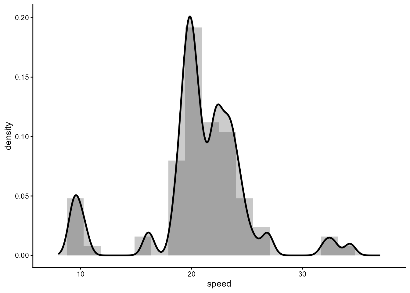
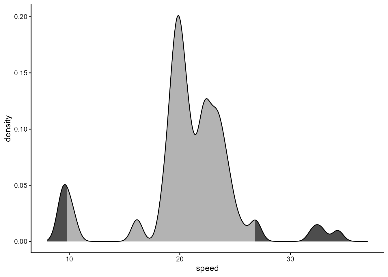
The quantiles can be highlighted similarly as in
stat_distrmix_area() using function
find_quantiles().
ggplot(data.frame(speed = galaxies * 1e-3), aes(x = speed)) +
  stat_density(
    aes(fill =
          after_stat(find_quantiles(density, quantiles = c(0.05, 0.95)) != 2)),
    bw = 0.5,
    geom = "area", outline.type = "upper",
    colour = "black",
    show.legend = FALSE) +
  scale_fill_grey(start = 0.7, end = 0.3) +
  expand_limits(x = c(8, 37))