Peaks and Valleys
‘ggpmisc’ 1.0.0.9000
Pedro J. Aphalo
2026-07-08
Source:vignettes/articles/peaks-and-valleys.Rmd
peaks-and-valleys.RmdAims of ‘ggpmisc’ and caveats
Package ‘ggpmisc’ makes it easier to add to plots created using ‘ggplot2’ annotations. It does this in part by wrapping existing functions. In this article I describe how to highlight and label peaks and labels in 2D plots of data.
To avoid confusion it is good to make clear what may seem obvious
to some: if no plot is needed, then there is no reason to use the ggplot
statistics from this package. The values shown as annotations are
computed using function find_peaks(), which builds onto
function splus2R::peaks().
It is also important to remember that in most cases data analysis including exploratory and other stages should take place before annotated plots for publication are produced. Even though data analysis can benefit from combined numerical and graphical representation of the results, the use I envision for ‘ggpmisc’ is mainly for the production of plots for publication or communication. In case case, whether used for analysis or communication, it is crucial that users cite and refer both to ‘ggpmisc’ and to the underlying R and R packages when publishing plots created with functions and methods from ‘ggpmisc’.
Preliminaries
We load all the packages used in the examples.
Attaching package ‘ggpmisc’ also attaches package ‘ggpp’, which provides some of the geometries and positions used in the examples below. Package ‘ggpp’ can be loaded and attached on its own, and has separate documentation.
As we will use text and labels on the plotting area we change the default theme to an uncluttered one.
Layer functions stat_peaks() and
stat_valleys()
Two statistics, stat_peaks() and
stat_valleys(), are described together in this section as
they are very similar. In the current implementation they do not support
fitting of peaks, and they simply find local or global, maxima and
minima. They require data to be mapped to aesthetics x and
y, with y being numeric and x,
numeric, time, datetime or date as supported by ‘ggplot2’.
They support flipping with an argument to orientation as in
‘ggplot2’ (>= 3.4.0).
These two statistics simplify/automate the labelling of peaks and valleys and add the possibility of ignoring some peaks or valleys based on their height or depth using thresholds. The role of arguments passed to different parameters is described in the help page. Here the focus is on explained examples of the different ways in which peaks and valleys can be annotated in plots.
Below the time series lynx and Nile are
used taking advantage of specializations of method ggplot()
defined in package ‘ggpp’, which automatically convert time series
stored in objects of classes ts or xts into
data frames. They by default also map time to the
x aesthetic and the observed variable to the y
aesthetic. An argument created by a call to aes() and
passed as argument to formal parameter mapping overrides
the default. Functions stat_peaks() and
stat_valleys() from package ‘ggpmisc’ can be used with
numeric, date or datetime values
mapped to x. An argument passed to parameter
orientation can be used to flip the data before the search
of peaks and valleys.
It can be of interest to locate peaks an valleys not only in time
series data, but also in spatial data, and other data indexed by a
regular sequence of values of the independent variable. Package ‘ggspectra’
implements variations
of stat_peaks() and stat_valleys() with
additional features useful with light and optical spectra while assuming
that the variable mapped to the x aesthetic described
wavelengths.
Plot p.lx0 is used as a base for several different
examples. Passing as.numeric = FALSE retains the variable
extracted from the time series as a datetime object while with
as.numeric = TRUE it is converted into
numeric. In this time series, the extracted time is a
variable of class Date.
p.lx0 <-
  ggplot(lynx, as.numeric = FALSE) +
  geom_line() +
  geom_point(shape = "circle small")

class(p.lx0$data$time)
#> [1] "Date"
class(p.lx0$data$lynx)
#> [1] "numeric"

p.lx0
By default stat_peaks() and stat_valleys()
use geom_point(), which when adding a layer after (= on
top) of the layers already added to p.lx0 with
geom_line() and geom_point() in the plot
overplots the observations corresponding to peaks. They can be made
visible by setting an aesthetic like colour,
size, shape, etc., to a different constant
value. Unless other geometries are used stat_peaks()
and stat_valleys() are added to plots after the layers
displaying all observations.
Minimal examples
Function stat_peaks() identifies maxima of
y.
p.lx0 +
  stat_peaks(colour = "red")
Similarly, function stat_valleys() identifies minima of
y.
p.lx0 +
  stat_valleys(colour = "blue")
Flipping the statistics’ orientation
As in many statistics from package ‘ggplot2’, these statistics from
package ‘ggpmisc’ support flipping by passing an argument to parameter
orientation. In this contrived example, years are mapped to
y and the number of lynx skins to x.
ggplot(lynx, aes(lynx, time)) +
  geom_line(orientation = "y") +
  geom_point(shape = "circle small") +
  stat_peaks(colour = "red", orientation = "y") +
  stat_valleys(colour = "blue", orientation = "y")
Moving-window span
Peaks and valleys are the maximum and minimum value within a moving
window. The width of the moving window as an odd number of observations
is controlled by the argument passed to formal parameter
span. Function stat_peaks() identifies the
global maximum or local maxima depending on the value of
span. With the default of span = 5 a moving
window of width 5 is used. Although suitable for lynx, the
default window width in most cases will need to be adjusted to the
characteristics of the data.
Passing span = NULL in the call results in a search for
the global maximum of y in a single window encompassing the
whole vector of values. (Passing span = Inf or any integer
larger than the length of the vector results in the same behaviour.)
p.lx0 +
  stat_peaks(colour = "red", span = NULL)
The cycle in the lynx time series is near 10, so using
span = 9 still detects the same peaks as with
span = 5 except for that for year 1915 as this peak is
never the taller than all of its neighbours in the wider moving
window.
p.lx0 +
  stat_peaks(colour = "red", span = 9)
With span = 51 stat_peaks() find only the
two tallest peaks.
p.lx0 +
  stat_peaks(colour = "red", span = 51)
Global height or depth threshold
Arguments passed to span worked well with the very
regular cycles and lack of major disturbances in the lynx
time series.
One approach to differentiate between major and minor peaks is to
require a minimum height for them. The most direct approach is to pass
an argument to global.threshold expressed in data units. We
indicate this with I() which sets class "AsIs"
in the numeric value passed as argument.
p.lx0 +
  stat_peaks(colour = "red", global.threshold = I(4300))
The same plot as above, annotated with the threshold value passed as
argument to global.threshold shown together with the range
of the data.

If we simply pass an unprotected numeric value in the
range 0\ldots1 this value is taken as
relative to the data range.
p.lx0 +
  stat_peaks(colour = "red", global.threshold = 0.66)
The same plot as above, annotated with the threshold value passed as
argument to global.threshold shown together with the range
of relative values accepted.

In the very unlikely cases of wanting to highlight only the shorter
peaks, a value in -1\ldots0 can be
passed as argument to global.threshold.
p.lx0 +
  stat_peaks(colour = "red", global.threshold = -0.66)
The threshold is highlighted with a red line and on the right side axis ticks show values expressed relative to the data range with a negative sign.

The threshold works similarly for valleys and peaks, with larger values making the selection more strict.
p.lx0 +
  stat_valleys(colour = "blue", global.threshold = 0.97)
In the annotated plot below, the value of the argument passed to
global.threshold is highlighted with a blue line. The range
of accepted relative threshold values is shown on the axis on the right,
in which tick labels go in the reverse direction compared to peaks.

Within window height and depth threshold
With a less regular time series with a superimposed trend or a change
point like the Nile series of water flow, span
and global.threshold are not able to separate prominent
narrow peaks from broader or less prominent ones.
p.nl0 <-
  ggplot(Nile, as.numeric = FALSE) +
  geom_line() +
  geom_point(shape = "circle small")

class(p.nl0$data$time)
#> [1] "Date"
class(p.nl0$data$Nile)
#> [1] "numeric"

p.nl0
With the default value of span = 5 some locally small
peaks are highlighted. Setting global.threshold would not
help as a change point around year 1900 makes it impossible to find a
suitable value.
p.nl0 +
  stat_peaks(colour = "red")
Parameter local.threshold makes it possible to add a
threshold to use within the moving window, using a reference computed at
each displacement of the window. The default is to compare the peak
height to the median height of the observations in the window. The local
threshold uses the same scaling as the global threshold: it is given as
relative to the range of the data.
Comparing to the median of the window tends to ignore the broader peaks.
p.nl0 +
  stat_peaks(colour = "red", local.threshold = 0.15)
The same plot as above, annotated. The running median for the same span is shown as a red dashed line. Peaks that are more than 0.15 relative units from the running median line are retained.

Using local.base = "farthest" test for the range of
values within the window, thus penalizing much less broad peaks as long
as they fit within the width of the window given by span.
The example below works well for the Nile time series.
p.nl0 +
  stat_peaks(colour = "red",
             local.threshold = 0.25,
             local.reference = "farthest")
The same plot as above, annotated. The running minimum for the same span is shown as a red dashed line. Peaks that are more than 0.25 relative units from the running minimum line are retained.

Local thresholds work for valleys in the same way as for peaks. A
larger value for local.threshold results in fewer valleys
highlighted.
p.nl0 +
  stat_valleys(colour = "blue", local.threshold = 0.15)
The same plot as above, annotated. The running median for the same span is shown as a blue dashed line. Peaks that are more than 0.15 relative units from the running median line are retained. The moving median line is the same as used for peaks, but the distance assessed for valleys is downwards from this line instead of upwards for peaks.

As shown above, the local.threshold argument is used
as is when the argument passed to local.reference
is "median" or "farthest", i.e., the same
distance between peak and reference is used for cut-off irrespective of
the value of the reference. In cases when the prominence of peaks is
positively correlated with the baseline, a local.threshold
that increases together with increasing local.reference
makes it possible to apply a less stringent height requirement when the
computed reference has a smaller value. Currently implemented (‘ggpmisc’
> 0.6.2) are natural logarithm and square root weighting with
"median.log", "farthest.log",
"median.sqrt", and "farthest.sqrt" as argument
for local.reference.
Labeling of peaks and valleys
The default mappings to aesthetics support additional geometries,
including geom_text() and geom_label(). In
this example the position, hjust and
angle arguments are passed along to the geom while the
x.label.format argument is handled by the statistic, to
create labels containing only the year component of variable
time. In the case of variables of class Date
like on this case, the format specification is that of function
strptime() as described in its documentation.
p.lx0 +
  stat_peaks(geom = "text",
             x.label.fmt = "%Y",
             position = position_nudge(y = 100),
             hjust = "left",
             angle = 90) +
  expand_limits(y = 8000)
The repulsive geoms from package ‘ggrepel’ are also specifically supported. The two stats handle this as a special case, returning the coordinates of all observations to ensure that they are not overlapped by repulsed text or labels.
p.lx0 +
  stat_peaks(geom = "text_repel",
             x.label.fmt = "%Y",
             position = position_nudge_keep(y = 100)) +
  expand_limits(y = 7500)
When calling stat_valleys(), what needs to be changed
compared to when calling stat_peaks() above is the
direction of the nudge applied, to push labels above peaks and below
valleys.
p.lx0 +
  stat_peaks(x.label.fmt = "%Y",
             geom = "text_repel",
             colour = "red",
             box.padding = 0.1,
             point.padding = 4,
             position = position_nudge_keep(y = 100)) +
  stat_peaks(colour = "red") +
  stat_valleys(x.label.fmt = "%Y",
               geom = "text_repel",
               colour = "blue",
               box.padding = 0.1,
               point.padding = 4,
               position = position_nudge_keep(y = -100)) +
  stat_valleys(colour = "blue") +
  expand_limits(y = c(-500, 7500))
As seen above, by default x-labels are mapped to aesthetic
label. Labels for y values at peaks are also
generated and can be mapped as usual. In the case of variables of mode
numeric, the format specification used is that of function
sprintf().
p.lx0 +
  stat_peaks(aes(label = after_stat(y.label)),
             y.label.fmt = "n=%i",
             geom = "text_repel",
             direction = "y",
             box.padding = 0.1,
             point.padding = 1,
             position = position_nudge_keep(y = 150),
             angle = 90) +
  stat_peaks(colour = "red") +
  expand_limits(y = 8200)
A mapping to the label aesthetic can be created with
function use_label().
p.lx0 +
  stat_peaks(use_label("x", "y", sep = " "),
             x.label.fmt = "%Y:",
             y.label.fmt = "%i",
             geom = "text_repel",
             direction = "y",
             box.padding = 0.1,
             point.padding = 1,
             position = position_nudge_keep(y = 150),
             angle = 90) +
  stat_peaks(colour = "red") +
  expand_limits(y = 9000)
It is also easy to combine x and y labels within a
call to aes(). Function paste() or any other
character string manipulation function can be used within a call to
aes() to “edit” the text to be added to the plot.
p.lx0 +
  stat_peaks(aes(label = after_stat(paste(x.label, y.label))),
             x.label.fmt = "%Y:",
             y.label.fmt = "%i",
             geom = "text_repel",
             direction = "y",
             box.padding = 0.1,
             point.padding = 1,
             position = position_nudge_keep(y = 150),
             angle = 90) +
  stat_peaks(colour = "red") +
  expand_limits(y = 9000)
The default mappings support geom_text(),
geom_label(), geom_rug(),
geom_hline() and geom_vline() from package
‘ggplot2’; geom_text_repel() and
geom_label_repel() from package ‘ggrepel’; and
geom_text_s(), geom_label_s() and
geom_vhline() from package ‘ggpp’. These and many other
geoms can be also used with mappings set with a call to
aes(). A few examples follow.
Using geom_rug() the position of the peaks can be shown
on the inside of the axis, and using position_nudge_to()
the text annotations can be moved next to them. Using
geom_text_repel() with direction = "x" we
enable horizontal repulsion and with
min.segment.length = Inf we disable the drawing of
connecting line segments.
p.lx0 +
  stat_peaks(x.label.fmt = "%Y",
             geom = "text_repel",
             size = 3.2,
             vjust = "top",
             min.segment.length = Inf,
             direction = "x",
             position = position_nudge_to(y = 7700)) +
  stat_peaks(geom = "rug",
             sides = "t") +
  expand_limits(y = 7500)
To use multiple geoms to annotate peaks, the stat must be called
multiple times, once for each geom. Passing span = NULL
sets the window where maxima are searched for to encompass the whole
data set, thus, only the global maximum and the global minimum are
annotated. A more elaborate label is assembled in a call to
paste() when specifying the aesthetic mapping with
aes(). geom_text_s() differs from
geom_text() in that a connecting segment is drawn together
with the text.
p.lx0 +
  stat_peaks(f_use_label("y", "x", format = "%s lynx skins in year %s"),             x.label.fmt = "%Y",
             y.label.fmt = "%i",
             span = NULL,
             geom = "text_s",
             hjust = "right",
             vjust = "bottom",
             colour = "red",
             box.padding = 0.1,
             point.padding = 4,
             position = position_nudge_keep(y = 200)) +
  stat_peaks(geom = "rug",
             span = NULL,
             colour = "red") +
  stat_peaks(span = NULL,
             geom = "hline",
             alpha = 1/5,
             colour = "red") +
  stat_valleys(f_use_label("y", "x", format = "%s lynx skins in year %s"),
               x.label.fmt = "%Y",
               y.label.fmt = "%i",
               span = NULL,
               geom = "text_s",
               hjust = "left",
               vjust = "top",
               colour = "blue",
               box.padding = 0.1,
               point.padding = 4,
               position = position_nudge_keep(y = -200)) +
  stat_valleys(geom = "rug",
               span = NULL,
               colour = "blue") +
  stat_valleys(span = NULL,
               geom = "hline",
               alpha = 1/5,
               colour = "blue") +
  expand_limits(y = c(-500, 7500))
With a few more tweaks we can modify the design of the annotations in
the plot above. To use geom_segment() we need to map a
constant to aesthetic xend.
p.lx0 +
  stat_peaks(f_use_label("y", "x", format = "%s lynx skins in year %s"),
             x.label.fmt = "%Y",
             y.label.fmt = "%i",
             span = NULL,
             geom = "text_s",
             vjust = "bottom",
             colour = "red",
             box.padding = 0.1,
             point.padding = 4,
             position = position_nudge_keep(y = 300)) +
  stat_peaks(span = NULL,
             geom = "segment",
             arrow = arrow(length = unit(2, "mm"), type = "closed"),
             xend = -Inf,
               alpha = 1/3,
             colour = "red") +
  stat_valleys(f_use_label("y", "x", format = "%s lynx skins in year %s"),
               x.label.fmt = "%Y",
               y.label.fmt = "%i",
               span = NULL,
               geom = "text_s",
               vjust = "top",
               colour = "blue",
               box.padding = 0.1,
               point.padding = 4,
               position = position_nudge_keep(y = -300)) +
  stat_valleys(span = NULL,
               geom = "segment",
               arrow = arrow(length = unit(2, "mm"), type = "closed"),
               xend = -Inf,
               alpha = 1/3,
               colour = "blue") +
  expand_limits(y = c(-500, 7500))
Functions find_peaks() and
find_valleys()
Function find_peaks(), is used internally in ‘ggpmisc’
to implement stat_peaks() and stat_valleys().
It can also be used on its own. Because of of the value expected by
scales’ breaks parameter, it is not possible to call this
function on the fly within a call to sec_axis() with the
plot data as an implicit argument. However, find_peaks()
can be used to generate vectors that can be passed as an argument to
parameter breaks. Below, to set breaks in the secondary
axes, we first create vectors of dates and numbers of lynx skins at the
peaks, and then use them as arguments in the call to
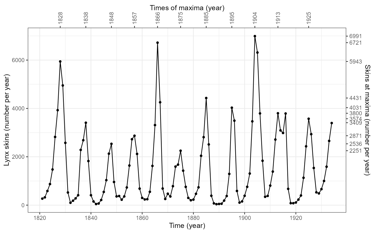
sec_axis(). Currently, there is no support for repulsion of
axis tick labels in packages ‘ggplot2’ or ‘legendry’, so to avoid
overlaps fewer peaks have to be annotated than in the plots above. The
use of span = 11, which is wider than the default
span = 5, to search for peaks results in the peak in year
1916, adjacent to that in year 1913, to be ignored.
lynx.tb <- try_tibble(lynx)
my.time.breaks <- lynx.tb$time[find_peaks(lynx.tb$x, span = 11)]
my.skins.breaks <- lynx.tb$x[find_peaks(lynx.tb$x, span = 11)]
p.lx0 +
  scale_x_date(name = "Time (year)",
               sec.axis = sec_axis(~ .,
                                   name = "Times of maxima (year)",
                                   breaks = my.time.breaks,
                                   labels = function(x) {strftime(x, "%Y")})) +
  scale_y_continuous(name = "Lynx skins (number per year)",
               sec.axis = sec_axis(~ .,
                                   name = "Skins at maxima (number per year)",
                                   breaks = my.skins.breaks)) +
  theme(axis.text.x.top = element_text(angle = 90, vjust = 0.5))
Of course, find_peaks() and find_valleys()
can be used to search for peaks and valleys independently of
plotting.
lynx[find_peaks(lynx)]
#>  [1] 5943 3409 2536  377 2871 6721  473 2251 4431 4031 6991 3800 3790 3574
time(lynx)[find_peaks(lynx)]
#>  [1] 1828 1838 1848 1851 1857 1866 1870 1875 1885 1895 1904 1913 1916 1925
Resources
Documentation for packages ggplot2, ggpp, ggrepel, and gginnards, as
well as the R Graphics Cookbook,
Learn R: As a Language and
ggplot2: Elegant Graphics for Data
Analysis books can help in finding/devising additional uses for
stat_peaks() and stat_valleys().