Custom Polynomial Models
‘ggpmisc’ 1.0.0.9000
Pedro J. Aphalo
2026-07-08
Source:vignettes/articles/poly-advanced.Rmd
poly-advanced.RmdAims of ‘ggpmisc’ and caveats
Package ‘ggpmisc’ makes it easier to add to plots created using ‘ggplot2’ annotations based on fitted models and other statistics. It does this by wrapping existing model fit and other functions. The same annotations can be produced by calling the model fit functions, extracting the desired estimates and adding them to plots. There are two advantages in wrapping these functions in an extension to package ‘ggplot2’: 1) we ensure the coupling of graphical elements and the annotations by building all elements of the plot using the same data and a consistent grammar and 2) we make it easier to annotate plots to the casual user of R, already familiar with the grammar of graphics.
To avoid confusion it is good to make clear what may seem obvious to some: if no plot is needed, then there is no reason to use this package. The values shown as annotations are not computed by ‘ggpmisc’ but instead by the usual model-fit and statistical functions from R and R packages. The same is true for model predictions, residuals, etc. that some of the functions in ‘ggpmisc’ display as lines, segments, or other graphical elements.
It is also important to remember that in most cases data analysis including exploratory and other stages should take place before annotated plots for publication are produced. Even though data analysis can benefit from combined numerical and graphical representation of the results, the use I envision for ‘ggpmisc’ is mainly for the production of plots for publication or communication. In case case, whether used for analysis or communication, it is crucial that users cite and refer both to ‘ggpmisc’ and to the underlying R and R packages when publishing plots created with functions and methods from ‘ggpmisc’.
Introduction
The first chapter gives examples of the use of the stats
from ‘ggpmisc’ for plotting predictions and annotating ggplots using
robust and resistant regression .
The second chapter gives examples of the use of the stats from
‘ggpmisc’ for plotting predictions and annotating ggplots with fitted
linear, cubic and polynomial splines. The third chapter gives examples
of the use of the stats from ‘ggpmisc’ for plotting predictions
and annotating ggplots with functions wrapping model fit methods
together with model selection and other code that can automate the
choice of the model formula, model fit method, etc., on a per data group
basis.
Fitted models in stat_poly_line() and
stat_poly_eq()
Both functions are designed for flexibility while still attempting to keep their implementation and use straightforward.
Function stat_poly_eq() returns a formatted string for
the fitted model equation only if the model formula is a
regular polynomial (with no missing intermediate power terms), with the
exception that the intercept can be missing. In all cases, all other
formatted string labels are still generated if the estimates are
available.
Function stat_poly_line() has fewer requirements for the
argument passed to formula. However, whether confidence
bands can be plotted for the fitted model lines depends on whether the
predict() method for the fitted model object computes them.
This is not the case for gls(), lme(),
nls(), onls() and several other model fit
functions. In many cases estimation of approximate confidence bands is
possible in R, one being through bootstrapping, which is computation
intensive. Bootstrapping can be implemented in user code using
boot() or with simpler code, for example, by methods
defined in R package ‘nlraa’. These approaches are currently not
supported by the layer functions in ‘ggpmisc’. In the case of
gls(), lme(), nls() and
onls() informative messages are issued if
se = TRUE is passed to stat_poly_line(), but
in other cases, errors with cryptic messages can be triggered in
‘ggplot2’ code.
Both stat_poly_eq() and
stat_poly_line():
- Accept any R function or its name as argument for
method, - as long as the fitted model object belongs to classes
"lm","rlm","lqs","lts"or"gls", as tested withinherits(), and additionally models of other classes as long as query methods are available. - The implementation of
stat_poly_eq()andstat_poly_line()tolerates some missing methods and fields in model fit objects and their summary, i.e., returningNA_real_or emptycharacterstrings depending on the case. - The formula used to construct the equation is, whenever possible,
extracted from the fitted model object. Only exceptionally, when this
approach fails, the formula passed as argument for
formulain the call is used with a warning.
This design makes it possible to use as method existing
model fit functions that return an object of one of the classes
specifically supported, wrapper functions that call such functions, or
in some other way return an object of a known class such as
"lm". Even model fit functions returning an object
belonging to an “unrecognised” class are supported, sometimes partially,
depending on the availability of compatible specializations of the
generic methods defined in R’s ‘stats’ package, such as,
summary(), coef(), predict(),
fitted(), AIC(), etc.
To showcase this, I explore in this article the use of contributed
and user defined model fit functions through examples. Several of the
examples use facets or grouping to demonstrate how the fitted models
method and formula can dynamically depend on
the data in each panel or data grouping in a ggplot. A model and method
selection approach based on the data can be also useful in the absence
of facets and/or groups, for example for dynamic reports or
dashboards.
Two frequently used model fit functions that return model fit objects
that require special handling to extract values are supported in
‘ggpmisc’ by specific statistics: stat_ma_line() and
stat_ma_eq() for mayor axis (MA) regression with package
‘lmodel2’, and stat_quant_line(),
stat_quant_band() and stat_quant_equation()
for quantile regression with package ‘quantreg’. Their use is documented
in the User Guide and their help pages.
Preliminaries
Other packages are loaded in the section they are used.
Attaching package ‘ggpmisc’ also attaches package ‘ggpp’ as it provides several of the geometries used by default in the statistics described below. Package ‘ggpp’ can be loaded and attached on its own, and has separate documentation.
As we will use text and labels on the plotting area we change the default theme to an uncluttered one.
Robust and resistant methods
We consider cases in which fitting linear models with ordinary least squares (OLS) as criterion is unsuitable.
In the case of outliers, many methods are available, and each fit
function usually also supports several variations within a class of
methods. User-supplied weights can be usefull, e.g., when the different
values in data are means computed from varying numbers of
observations. Weights can be also computed, for example by assuming a
given distribution for errors, and decreasing the weight given in model
fitting to the “unusual/unlikely” observations. In robust
regression the weight given to the residuals for these observations
in the computation of the penalty function is decreased compared to OLS
with the effect of such decrease described as weights ranging
continuously between 0 and 1. In resistant regression, some
observations are ignored altogether, which is equivalent to discrete
weights taking one of two values, 0 or 1, and model fitted by, e.g., OLS
to the retained observations. There are other approaches, including
variance covariates, in which weights can be outside the 0 to 1 range.
There is not even consistency on wether weights enter as
multipliers or divisors in computtaions. One important departure is in
the weights returned by methods from package ‘lnme’.
Prior numerical weights are passed by mapping a variable to
the weight aesthetic (and used as argument to the
weights parameter of model fit funcitons).
Posterior weights are computed in connection with the fitting
of the model, sometimes by comparison to OLS.
Even if these approaches work “automatically”, similarly as when
discarding observations manually, it is important to investigate the
origin of outliers, and which observations are bing ignored or
down-weighted during model fitting. To ensure reproducibility and
interpretability it is crucial to report the results of analyses clearly
showing the weights used for different observations. For this reason
stat_poly_line() and stat_fit_deviations() in
‘ggpmisc’ (>= 0.7.0) include in the returned data
objects (the input to geoms) whenever they are available, both
prior weights and posterior
posterior.weights. The former being those passed by mapping
a variable to the weight aesthetic and used as argument for
the weights parameter of model fit function, and the latter
being those actually used, and possibly computed during model
fitting.
Robust regression (‘MASS’)
print(citation(package = "MASS", auto = TRUE), bibtex = FALSE)
#> To cite package 'MASS' in publications use:
#>
#>   Ripley B, Venables B (2025). _MASS: Support Functions and Datasets
#>   for Venables and Ripley's MASS_. doi:10.32614/CRAN.package.MASS
#>   <https://doi.org/10.32614/CRAN.package.MASS>. R package version
#> 7.3-65, <https://CRAN.R-project.org/package=MASS>.Package ‘MASS’ provides function rlm() for “Robust
Fitting of Linear Models”. The returned value is an "rlm"
object. Class "rlm" is derived from "lm" so
the stats work mostly as expected. However, we need to be aware that no
R^2 or P estimates are available and the
corresponding labels are empty strings.
The first example plot is in the style I recommend for use in reporting as it makes the weights visible, later plots from this same subset of the data are mostly useful in teaching and data exploration.
ggplot(subset(mpg, class == "suv"), aes(displ, hwy)) +
  stat_poly_line(method = "rlm") +
  stat_poly_eq(use_label("eq", "n", "method"),
               label.x = "right",
               method = "rlm") +
  stat_fit_deviations(method = "rlm",
                      mapping = aes(colour = after_stat(posterior.weights)),
                      show.legend = TRUE,
                      geom = "point") +
  scale_color_gradient(low = "red", high = "blue", limits = c(0, 1)) +
  theme(legend.position = "top")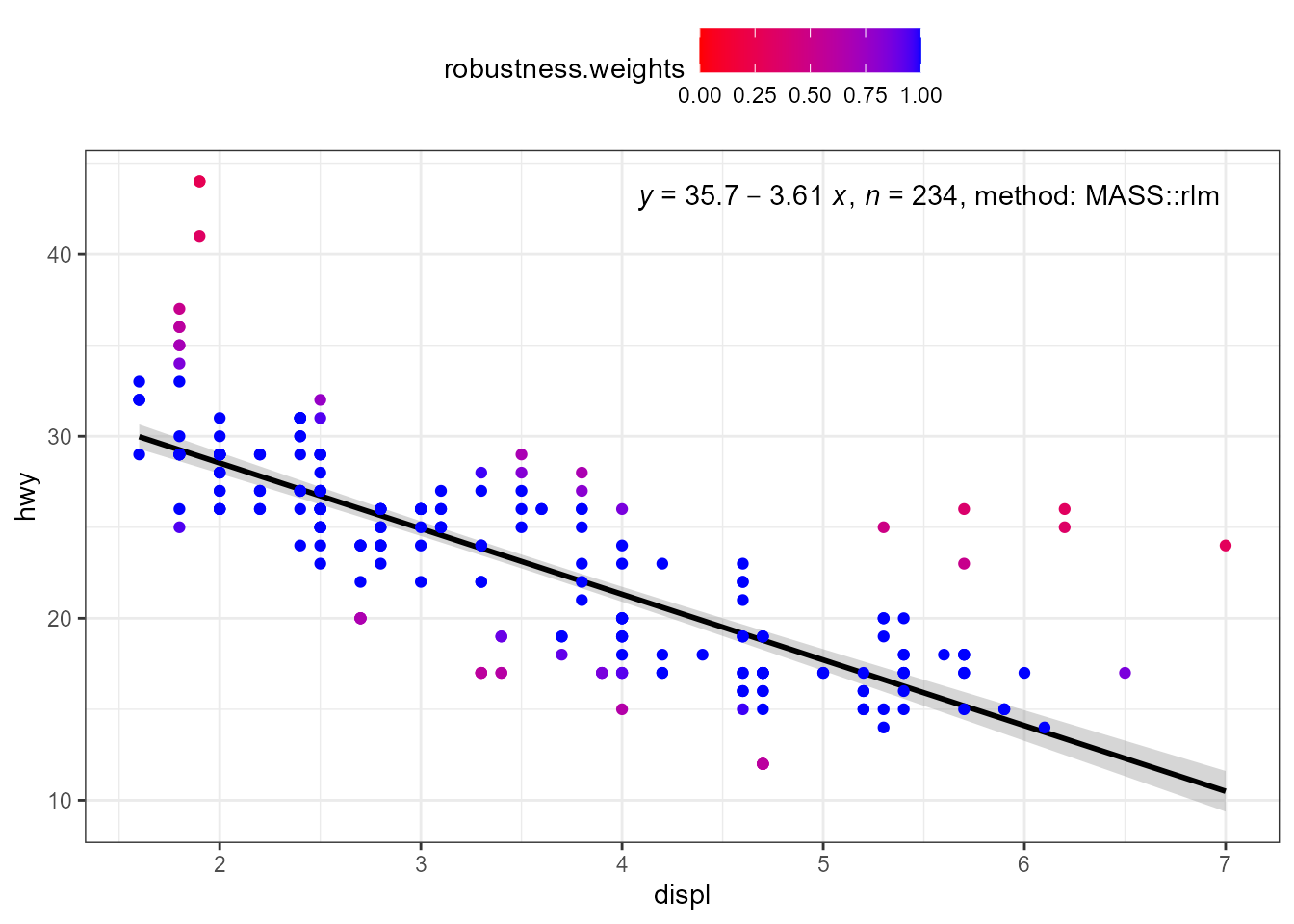
Fitted values and deviations highlighted.
ggplot(subset(mpg, class == "suv"), aes(displ, hwy)) +
  stat_poly_line(method = "rlm") +
  stat_fit_fitted(method = "rlm", shape = "cross") +
  stat_fit_deviations(method = "rlm", linewidth = 0.3) +
  stat_fit_deviations(method = "rlm",
                      mapping = aes(colour = after_stat(posterior.weights)),
                      show.legend = TRUE,
                      geom = "point")+
  scale_color_gradient(low = "red", high = "blue", limits = c(0, 1)) +
  theme(legend.position = "top")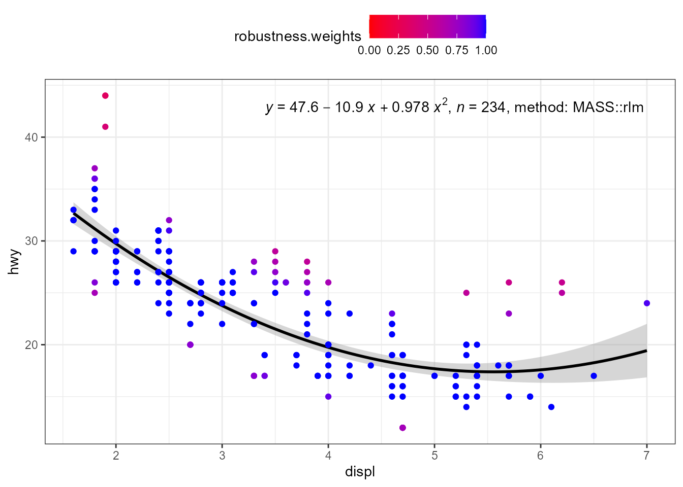
Residuals plotted.
ggplot(subset(mpg, class == "suv"), aes(displ, hwy)) +
  geom_hline(yintercept = 0, linetype = "dotted") +
  stat_fit_residuals(method = "rlm",
                     resid.type = "response",
                     mapping = aes(colour = after_stat(posterior.weights)),
                     show.legend = TRUE,
                     geom = "point") +
  labs(y = "Response residuals") +
  scale_color_gradient(low = "red", high = "blue", limits = c(0, 1)) +
  theme(legend.position = "top")
ggplot(subset(mpg, class == "suv"), aes(displ, hwy)) +
  geom_hline(yintercept = 0, linetype = "dotted") +
  stat_fit_residuals(method = "rlm",
                     resid.type = "pearson",
                     mapping = aes(colour = after_stat(posterior.weights)),
                     show.legend = TRUE,
                     geom = "point") +
  labs(y = "Pearson residuals") +
  scale_color_gradient(low = "red", high = "blue", limits = c(0, 1)) +
  theme(legend.position = "top")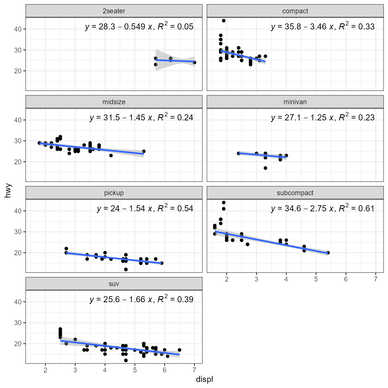
We are not constrained to a first degree polynomial. This plot follows the recommended style for reporting.
my.formula <- y ~ poly(x, 2, raw = TRUE)
ggplot(subset(mpg, class == "suv"), aes(displ, hwy)) +
  stat_poly_eq(use_label("eq", "n", "method"),
               formula = my.formula,
               label.x = "right",
               method = "rlm") +
  stat_poly_line(method = "rlm",
                 formula = my.formula,
                 colour = "black") +
  stat_fit_deviations(mapping = aes(colour = after_stat(posterior.weights)),
                      method = "rlm",
                      formula = my.formula,
                      show.legend = TRUE,
                      geom = "point") +
  scale_color_gradient(low = "red", high = "blue", limits = c(0, 1)) +
  theme(legend.position = "top")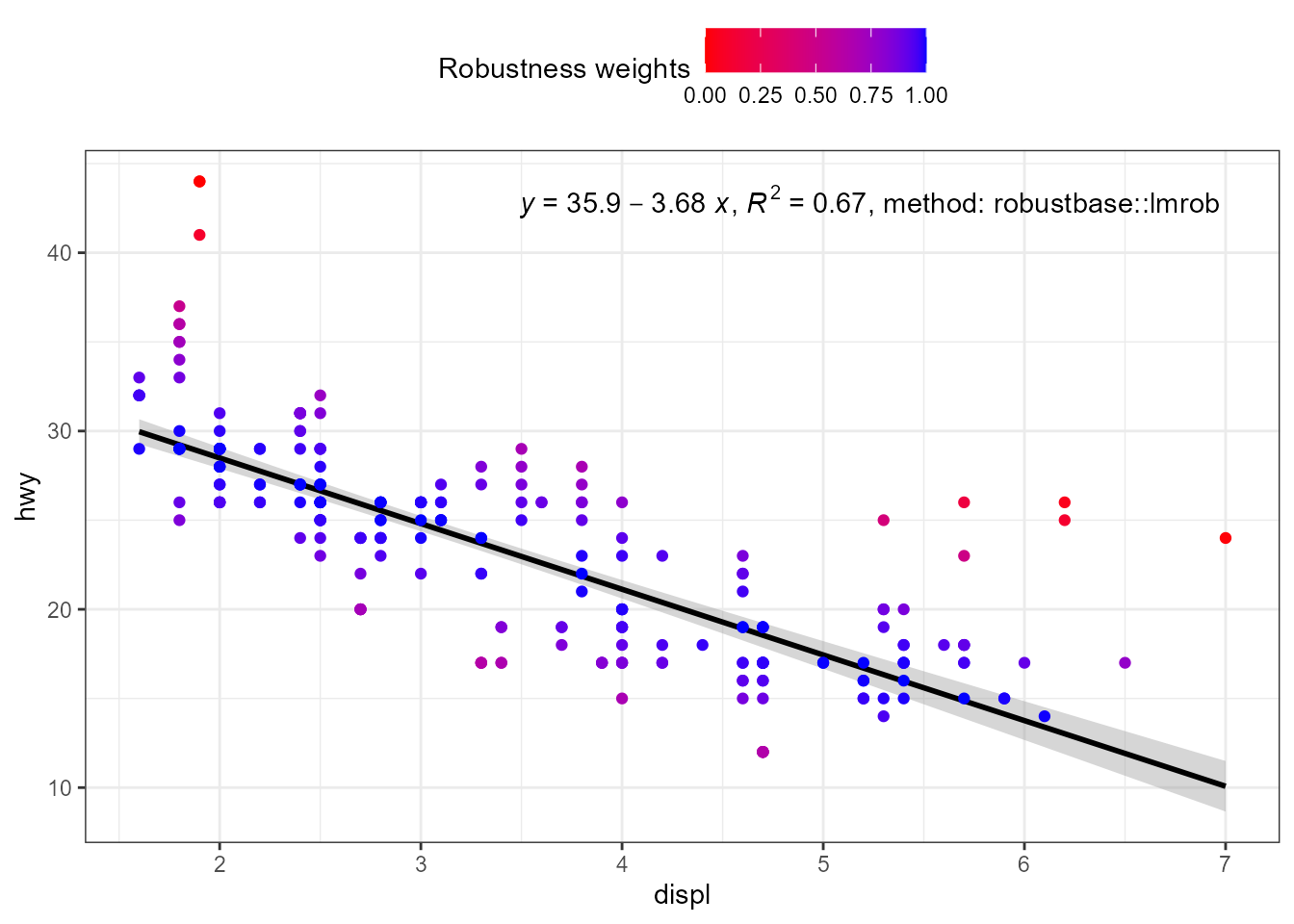
We can the same approach with the whole data set using facets.
ggplot(mpg, aes(displ, hwy)) +
  stat_poly_line(method = "rlm") +
  stat_poly_eq(method = "rlm", mapping = use_label("eq", "n"),
               label.x = "right") +
    stat_fit_deviations(method = "rlm",
                      mapping = aes(colour = after_stat(posterior.weights)),
                      show.legend = TRUE,
                      geom = "point") +
  facet_wrap(~class, ncol = 2) +
  scale_color_gradient(low = "red", high = "blue", limits = c(0, 1)) +
  theme(legend.position = "top")
Robust regression (‘robustbase’)
print(citation(package = "robustbase", auto = TRUE), bibtex = FALSE)
#> To cite package 'robustbase' in publications use:
#>
#>   Maechler M, Todorov V, Ruckstuhl A, Salibian-Barrera M, Koller M,
#>   Conceicao EL (2026). _robustbase: Basic Robust Statistics_.
#>   doi:10.32614/CRAN.package.robustbase
#>   <https://doi.org/10.32614/CRAN.package.robustbase>. R package version
#> 0.99-7, <https://CRAN.R-project.org/package=robustbase>.Package ‘robustbase’ provides function lmrob() for
“MM-type Estimators for Linear Regression”. The returned value is a
"lmrob" object. Class "lmrob" is derived from
"lm" so the stats work mostly as expected. However, we need
to be aware that no P estimate is
available and the corresponding labels are empty strings.
A few examples are given, as the only change to the code from the
previous section is in the argument passed to parameter
method. The first plot is what I consider suitable for use
in reports. Using defaults, lmrob seems to be more
aggresive against “outliers” than rlm, at least for these
data.
ggplot(subset(mpg, class == "suv"), aes(displ, hwy)) +
  stat_poly_line(method = "lmrob") +
  stat_poly_eq(use_label("eq", "n", "method"),
               label.x = "right",
               method = "lmrob") +
  stat_fit_deviations(method = "lmrob",
                      mapping = aes(colour = after_stat(posterior.weights)),
                      show.legend = TRUE,
                      geom = "point") +
  scale_color_gradient(low = "red", high = "blue", limits = c(0, 1)) +
  theme(legend.position = "top")
Fitted values and deviations highlighted.
ggplot(subset(mpg, class == "suv"), aes(displ, hwy)) +
  stat_poly_line(method = "lmrob") +
  stat_fit_fitted(method = "lmrob", shape = "cross") +
  stat_fit_deviations(method = "lmrob", linewidth = 0.3) +
  stat_fit_deviations(method = "lmrob",
                      mapping = aes(colour = after_stat(posterior.weights)),
                      show.legend = TRUE,
                      geom = "point")+
  scale_color_gradient(low = "red", high = "blue", limits = c(0, 1)) +
  theme(legend.position = "top")
Residuals plotted.
ggplot(subset(mpg, class == "suv"), aes(displ, hwy)) +
  geom_hline(yintercept = 0, linetype = "dotted") +
  stat_fit_residuals(method = "lmrob",
                     resid.type = "response",
                     mapping = aes(colour = after_stat(posterior.weights)),
                     show.legend = TRUE,
                     geom = "point") +
  labs(y = "Response residuals") +
  scale_color_gradient(low = "red", high = "blue", limits = c(0, 1)) +
  theme(legend.position = "top")
Resistant regression (‘robustbase’)
print(citation(package = "robustbase", auto = TRUE), bibtex = FALSE)
#> To cite package 'robustbase' in publications use:
#>
#>   Maechler M, Todorov V, Ruckstuhl A, Salibian-Barrera M, Koller M,
#>   Conceicao EL (2026). _robustbase: Basic Robust Statistics_.
#>   doi:10.32614/CRAN.package.robustbase
#>   <https://doi.org/10.32614/CRAN.package.robustbase>. R package version
#> 0.99-7, <https://CRAN.R-project.org/package=robustbase>.Package ‘robustbase’ provides function ltsReg() for
“least trimmed squares” regression. The returned value is an
"lts" object. The usual accessors functions are available
for Class "lts".
Package ‘MASS’ provides function lqs() for “Resistant
Regression”. The recommended method for this function is
"lts". Thus, using function ltsReg() from
package ‘robustbase’ is preferable as not all the usual accessors are
available when using lqs(). If needed, lqs()
is also, partly supported by ‘ggpmisc’, but no example is shown.
A few examples are given, as the only change to the code from the
previous sections is in the argument passed to parameter
method. The first plot is what I consider suitable for use
in reports.
ggplot(subset(mpg, class == "suv"), aes(displ, hwy)) +
  stat_poly_line(method = "lts") +
  stat_poly_eq(use_label("eq", "n", "method"),
               label.x = "right",
               method = "lts") +
  stat_fit_deviations(method = "lts",
                      mapping = aes(colour = after_stat(posterior.weights)),
                      show.legend = TRUE,
                      geom = "point") +
  scale_color_gradient(low = "red", high = "blue", limits = c(0, 1)) +
  theme(legend.position = "top")
#> Fitted line plotted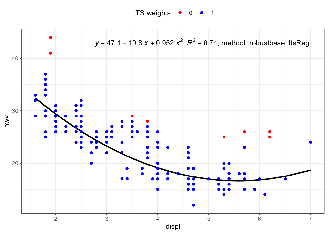
Fitted values and deviations highlighted.
ggplot(subset(mpg, class == "suv"), aes(displ, hwy)) +
  stat_poly_line(method = "lts") +
  stat_fit_fitted(method = "lts", shape = "cross") +
  stat_fit_deviations(method = "lts", linewidth = 0.3) +
  stat_fit_deviations(method = "lts",
                      mapping = aes(colour = after_stat(posterior.weights)),
                      show.legend = TRUE,
                      geom = "point")+
  scale_color_gradient(low = "red", high = "blue", limits = c(0, 1)) +
  theme(legend.position = "top")
#> Fitted line plotted
Residuals plotted.
ggplot(subset(mpg, class == "suv"), aes(displ, hwy)) +
  geom_hline(yintercept = 0, linetype = "dotted") +
  stat_fit_residuals(method = "lts",
                     mapping = aes(colour = after_stat(posterior.weights)),
                     show.legend = TRUE,
                     geom = "point") +
  labs(y = "Response residuals") +
  scale_color_gradient(low = "red", high = "blue", limits = c(0, 1)) +
  theme(legend.position = "top")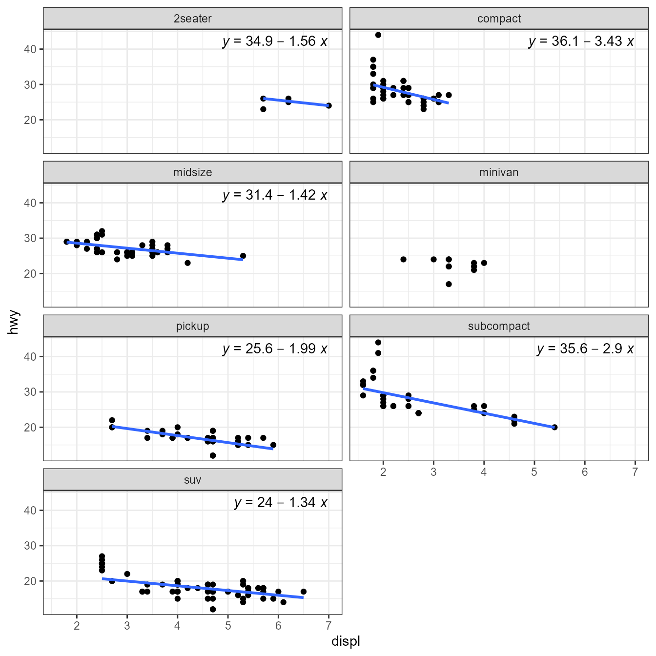
In the examples above the argument passed was
method = "lts", which is a convenience short notation
equivalent to method = robustbase::ltsReg.
Use of variance covariates
Generalised least squares (GLS) is an extension to OLS that makes it possible to describe how the variance of the response y varies. GLS supports description of heterogeneous variance by means of variance covariates and correlation structures.
General Least Squares (‘nlme’)
print(citation(package = "nlme", auto = TRUE), bibtex = FALSE)
#> To cite package 'nlme' in publications use:
#>
#>   Pinheiro J, Bates D, R Core Team (2026). _nlme: Linear and Nonlinear
#>   Mixed Effects Models_. doi:10.32614/CRAN.package.nlme
#>   <https://doi.org/10.32614/CRAN.package.nlme>. R package version
#> 3.1-169, <https://CRAN.R-project.org/package=nlme>.In ‘ggpmisc’ (>= 0.6.2) function gls() from package
‘nlme’ is supported natively by functions stat_poly_line()
and stat_poly_eq(). In this example, using a variance
covariate. Currently, support is limited to the prediction line, and
labels.
ggplot(subset(mpg, class == "suv"), aes(displ, hwy)) +
   geom_point() +
   stat_poly_line(method = "gls",
                  method.args = list(weights = nlme::varPower())) +
   stat_poly_eq(method = "gls",
                method.args = list(weights = nlme::varPower()),
                mapping = use_label("eq", "n", "method"),
   label.x = "right")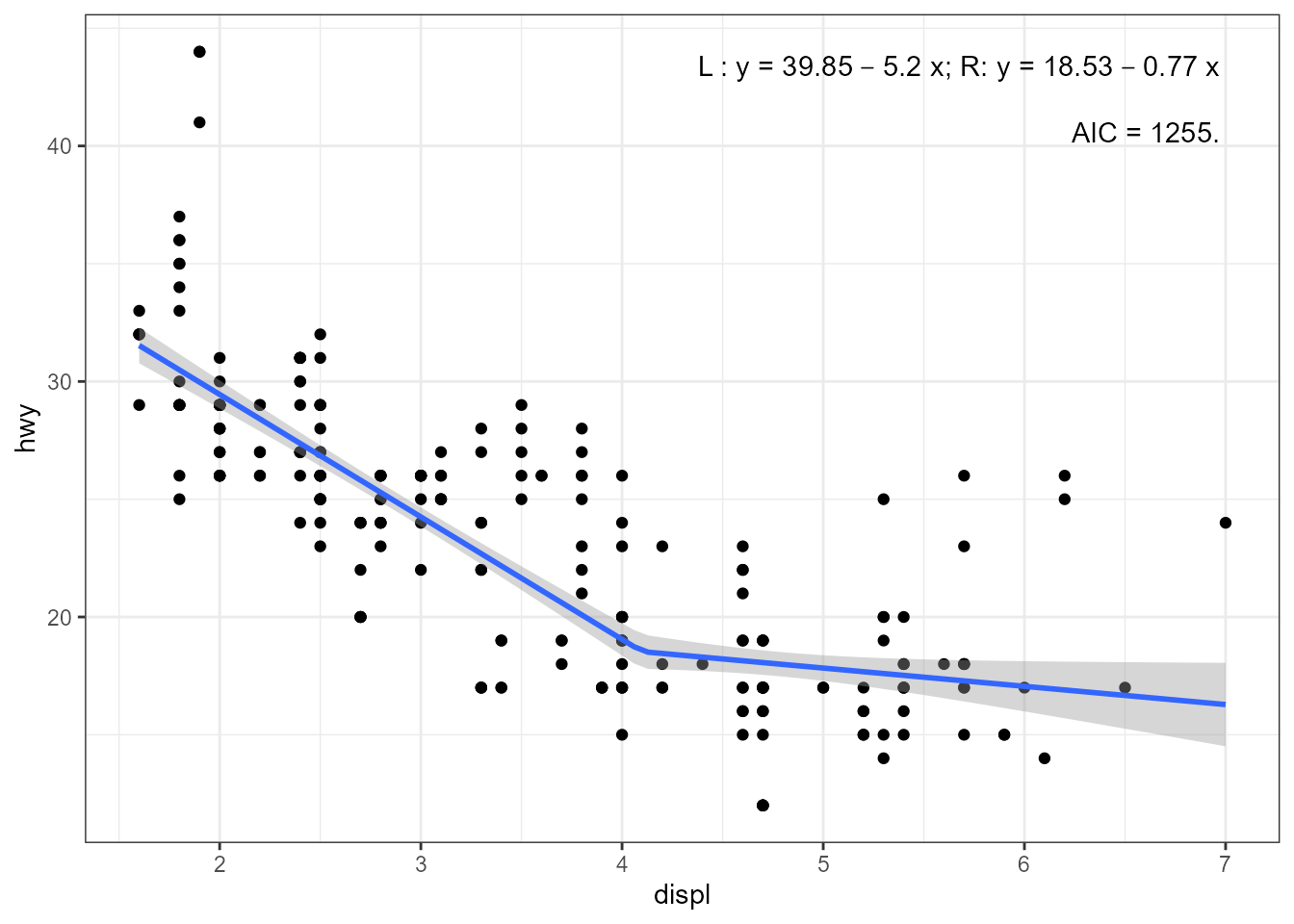
Fitted values and deviations highlighted. Posterior weights, in this case fitted using a power of variance covariate are not values in the range between 0 and 1 as in robust and resistant regression approaches. Thus, their interpretation is different. In this example instead of mapping the weights to the colour of points, we map them to the segments.
ggplot(subset(mpg, class == "suv"), aes(displ, hwy)) +
  stat_poly_line(method = "gls",
                 method.args = list(weights = nlme::varPower())) +
  stat_fit_fitted(method = "gls",
                  method.args = list(weights = nlme::varPower()),
                  shape = "cross") +
  stat_fit_deviations(method = "gls",
                  method.args = list(weights = nlme::varPower()),
                  linewidth = 0.3,
                  mapping = aes(colour = after_stat(posterior.weights))) +
  geom_point()
Residuals plotted.
ggplot(subset(mpg, class == "suv"), aes(displ, hwy)) +
  geom_hline(yintercept = 0, linetype = "dotted") +
  stat_fit_residuals(method = "gls",
                     method.args = list(weights = nlme::varPower()),
                     resid.type = "response",
                     mapping = aes(colour = after_stat(posterior.weights))) +
  labs(y = "Response residuals")
ggplot(subset(mpg, class == "suv"), aes(displ, hwy)) +
  geom_hline(yintercept = 0, linetype = "dotted") +
  stat_fit_residuals(method = "gls",
                     method.args = list(weights = nlme::varPower()),
                     resid.type = "pearson",
                     mapping = aes(colour = after_stat(posterior.weights))) +
  labs(y = "Pearson residuals")
ggplot(subset(mpg, class == "suv"), aes(displ, hwy)) +
  geom_hline(yintercept = 0, linetype = "dotted") +
  stat_fit_residuals(method = "gls",
                     method.args = list(weights = nlme::varPower()),
                     resid.type = "normalized",
                     mapping = aes(colour = after_stat(posterior.weights))) +
  labs(y = "Normalized residuals")
Splines
Splines are used when a flexible curve is required to efficiently describe a relationship between variables. Splines are composed of segments connected at knots. The simplest possible are linear splines where each segment is a straight line. In higher degree splines the segments are polynomials and conditions are imposed to ensure continuity at knots even for their derivative, to ensure smooth transition at each not. Except for linear splines the fitted parameters for each segment and not locations are too complex to be informative.
Even when model fit equations are not useful or are not generated
automatically, other labels constructed by stat_poly_eq()
remain useful. This stat not only returns ready made labels but also
numeric values for parameter estimates.
The approach to splines described here is that using base functions
within the model formula. This approach makes it possible
to use existing model fitting functions such as lm() for
linear models, to fit models that include terms that describe
splines.
Linear Splines (‘lspline’)
print(citation(package = "lspline", auto = TRUE), bibtex = FALSE)
#> To cite package 'lspline' in publications use:
#>
#>   Bojanowski M (2017). _lspline: Linear Splines with Convenient
#>   Parametrisations_. doi:10.32614/CRAN.package.lspline
#>   <https://doi.org/10.32614/CRAN.package.lspline>. R package version
#>   1.0-0, <https://CRAN.R-project.org/package=lspline>.
library(lspline)Package ‘lspline’ provides base functions that can be used to fit
linear splines. In this first example function lm() is
used. Spline base functions are included as terms in the model formula.
The functions from package ‘lspline’ do not fit the change points where
the knots are located. Functions, lspline(),
qlspline() amd elspline() can be used directly
in the model formula passed to stat_poly_line(). They can
be used also with stat_poly_eq() but no equation label is
returned. Thus, it is necessary to construct in the call to
aes() the equations for the different segments. Other
character labels are generated normally.
cp <- 4.1 # a guess
my.formula <- y ~ lspline::lspline(x, knots = cp)

ggplot(mpg, aes(displ, hwy)) +
  geom_point() +
  stat_poly_eq(aes(label =
                     after_stat(
                       paste("\"L : \"*y~`=`~", round(b_0, 2),
                           round(b_1, 2), "~x*\"; R: \"*y~`=`~",
                           round(b_0 + cp * b_1, 2),
                           round(b_2, 2), "~x",
                           sep = ""))),
               parse = TRUE, output.type = "numeric",
               label.x = "right",
               formula = my.formula,
               method = "lm") +
  stat_poly_eq(use_label("R2", "P", "AIC"),
               label.x = "right",
               label.y = 0.87,
               formula = my.formula,
               method = "lm") +
  stat_poly_line(method = "lm",
                 formula = my.formula)
Plotting fitted values and observations.
ggplot(mpg, aes(displ, hwy)) +
  stat_poly_line(method = "lm",
                 formula = my.formula) +
  geom_point() +
  stat_fit_fitted(method = "lm", formula = my.formula,
                  shape = "cross", alpha = 0.5)
Adding deviations.
ggplot(mpg, aes(displ, hwy)) +
  stat_poly_line(method = "lm",
                 formula = my.formula) +
  geom_point() +
  stat_fit_deviations(method = "lm",
                      formula = my.formula,
                      linewidth = 0.25) +
  stat_fit_fitted(method = "lm", formula = my.formula,
                  shape = "cross", alpha = 0.5)
Plotting residuals.
ggplot(mpg, aes(displ, hwy)) +
  geom_hline(yintercept = 0, linetype = "dotted") +
  stat_fit_residuals(method = "lm",
                     formula = my.formula) +
  labs(y = "Response residuals")
It is possible to use rlm() or lmrob()
instead of lm(), i.e., a robust approach instead of OLS.
Here we use method = "lmrob", combining the approach from
the example of robust regression with the linear spline fitting
above.
cp <- 4.1
my.formula <- y ~ lspline(x, knots = cp)

ggplot(mpg, aes(displ, hwy)) +
  stat_fit_deviations(formula = my.formula,
                      method = "lmrob",
                      mapping = aes(colour = after_stat(posterior.weights)),
                      show.legend = TRUE,
                      geom = "point") +
  stat_poly_eq(aes(label =
                     after_stat(
                     paste("\"L : \"*y~`=`~", round(b_0, 2),
                           round(b_1, 2), "~x",
                           "*\"; R: \"*y~`=`~",
                           round(b_0 + cp * b_1, 2),
                           round(b_2, 2), "~x",
                           sep = ""))),
               parse = TRUE,
               output.type = "numeric",
               label.x = "right",
               formula = my.formula,
               method = "lmrob") +
  stat_poly_eq(use_label("R2", "n", "method"),
               label.x = "right",
               label.y = 0.87,
               formula = my.formula,
               method = "lmrob") +
  stat_poly_line(method = "lmrob",
                 formula = my.formula) +
  scale_color_gradient(low = "red", high = "blue", limits = c(0, 1)) +
  theme(legend.position = "top")
Plotting residuals.
ggplot(mpg, aes(displ, hwy)) +
  geom_hline(yintercept = 0, linetype = "dotted") +
  stat_fit_residuals(method = "lmrob",
                     formula = my.formula,
                     mapping = aes(colour = after_stat(posterior.weights)),
                     show.legend = TRUE) +
  scale_color_gradient(name = "Weights",
                       low = "red", high = "blue",
                       limits = c(0, 1),
                       guide = "colourbar")
Linear Splines (‘segmented’)
Package ‘segmented’ has a design that makes it easy to use with
‘ggpmisc’. The splines are fitted with a special model fitting function.
The fitted model used has a structure consistent with that returned by
lm(). Any differences are smoothed by query/extract
functions that are consistent with those for "lm" objects.
As segmented linear models are not polynomials, no eq.label
is automatically generated. Another difference compared to
lspline(), described above, is that the location of change
points is estimated and returned. Starting from ‘ggpmisc’ (>= 0.6.3)
the estimates of the change point are returned by
stat_poly_eq() and can be used in user-assembled
model-“equation”- and other labels as shown in the examples below.
print(citation(package = "segmented", auto = TRUE), bibtex = FALSE)
#> To cite package 'segmented' in publications use:
#>
#>   Muggeo VMR (2026). _segmented: Regression Models with Break-Points /
#>   Change-Points Estimation (with Possibly Random Effects)_.
#>   doi:10.32614/CRAN.package.segmented
#>   <https://doi.org/10.32614/CRAN.package.segmented>. R package version
#>   2.2-1, <https://CRAN.R-project.org/package=segmented>.
library(segmented)Function segreg() makes it possible to fit LM and GLM
models that are segmented. Differently to ‘lspline’, the location of the
change points or spline knots is estimated during model fitting in
addition to estimating segment slopes and intercept. As ‘lspline’ it
uses a model formula to set the model including control of the
segmentation through seg(). Differently to
lspline(), segreg() is a model fit function
that returns a fitted model object with additional information on change
points and slopes.
The model formula = y ~ seg(x, npsi = 1) requests a fit
with a single change point, which being the default is equivalent to
formula = y ~ seg(x).
my.formula <- y ~ seg(x, npsi = 1)

ggplot(mpg, aes(displ, hwy)) +
  stat_poly_line(method = "segreg",
                 formula = my.formula)+
  geom_point() +
  stat_poly_eq(aes(label =
                     after_stat(
                       paste("x[cp]~`=`~",
                             round(knots[[1]][1], 2), " %+-% ",
                             round(knots.se[[1]][1], 2), "*\"; L: \"*y~`=`~",
                             round(b_0, 2), # "+",
                             round(b_1, 2), "~x*\"; R: \"*y~`=`~",
                             round(b_0 + knots[[1]][1] * (b_1 - b_2), 2),"+",
                             round(b_2, 2), "~x",
                             sep = ""))),
               parse = TRUE,
               output.type = "numeric",
               label.x = "right",
               formula = my.formula,
               method = "segreg") +
  stat_poly_eq(use_label("R2", "P", "AIC"),
               label.x = "right",
               label.y = 0.87,
               formula = my.formula,
               method = "segreg")
In the next example the slope of the second segment is fixed at zero
to keep it horizontal using
formula = y ~ seg(x, npsi = 1, est = c(1, 0)) where 1
indicates a fitted slope and 0 a slope fixed at this value. Because of
how the parameters are returned, the code to assemble the equation needs
to be rewritten.
my.formula <- y ~ seg(x, npsi = 1, est = c(1, 0))

ggplot(mpg, aes(displ, hwy)) +
  stat_poly_line(method = "segreg",
                 formula = my.formula) +
  geom_point() +
  stat_poly_eq(aes(label =
                     paste("x[cp]~`=`~",
                           round(after_stat(knots)[[1]][1], 2),
                           " %+-% ",
                           round(after_stat(knots.se)[[1]][1], 2),
                           "*\"; L: \"*y~`=`~",
                           round(after_stat(b_1), 2), # "+",
                           round(after_stat(b_2), 2), "~x",
                           "*\"; R: \"*y~`=`~",
                           round(after_stat(b_1) +
                                   after_stat(knots)[[1]][1] *
                                   after_stat(b_2),
                                 2),
                           sep = "")),
               parse = TRUE, output.type = "numeric",
               label.x = "right",
               formula = my.formula,
               method = "segreg") +
  stat_poly_eq(use_label("R2", "P", "AIC"),
               label.x = "right",
               label.y = 0.87,
               formula = my.formula,
               method = "segreg")
Highlighting fitted values.
ggplot(mpg, aes(displ, hwy)) +
  stat_poly_line(method = "segreg",
                 formula = my.formula) +
  geom_point() +
  stat_fit_fitted(method = "segreg",
                 formula = my.formula,
                 shape = "cross")
Plot of residuals.
ggplot(mpg, aes(displ, hwy)) +
  geom_hline(yintercept = 0, linetype = "dotted") +
  stat_fit_residuals(method = "segreg",
                      formula = my.formula)
Natural cubic splines (‘splines’)
Note: The lines for cubic and other smoothing
splines can be also added to plots with stat_smooth() from
package ‘ggplot2’.
print(citation(package = "splines", auto = TRUE), bibtex = FALSE)
#> The 'splines' package is part of R.  To cite R in publications use:
#>
#>   R Core Team (2026). _R: A Language and Environment for Statistical
#>   Computing_. R Foundation for Statistical Computing, Vienna, Austria.
#>   doi:10.32614/R.manuals <https://doi.org/10.32614/R.manuals>.
#>   <https://www.R-project.org/>.
#>
#> We have invested a lot of time and effort in creating R, please cite it
#> when using it for data analysis. See also 'citation("pkgname")' for
#> citing R packages.
library(splines)Package ‘splines’, part of the R distribution, provides function
ns() that can be used to fit natural splines. The approach
used in ‘splines’ is the same as described above for ‘lspline’,
ns() is added as a term in the model formula
passed to model fit functions such as lm(). Function
ns() can be part of the model formula passed to
stat_poly_line() and stat_poly_eq(). However,
stat_poly_eq() does not return a ready formatted character
label for the model equation, while other formatted character labels are
generated as for polynomials.
cp <- 4.1 # a guess
my.formula <- y ~ splines::ns(x, knots = cp)

ggplot(mpg, aes(displ, hwy)) +
  stat_poly_line(method = "lm",
                 formula = my.formula) +
  geom_point() +
  stat_poly_eq(use_label("R2", "P", "AIC"),
               label.x = "right",
               formula = my.formula,
               method = "lm")
Plotting fitted values and observations.
ggplot(mpg, aes(displ, hwy)) +
  stat_poly_line(method = "lm",
                      formula = my.formula) +
  geom_point() +
  stat_fit_fitted(method = "lm", formula = my.formula,
                  shape = "cross", alpha = 0.5)
Plotting residuals.
ggplot(mpg, aes(displ, hwy)) +
  geom_hline(yintercept = 0, linetype = "dotted") +
  stat_fit_residuals(method = "lm",
                     formula = my.formula) +
  labs(y = "Residuals")
It is possible to use rlm() or lmrob()
instead of lm(), for resistant and robust approaches to the
fitting of splines.
cp <- 4.1
my.formula <- y ~ splines::ns(x, knots = cp)

ggplot(mpg, aes(displ, hwy)) +
  stat_fit_deviations(formula = my.formula,
                      method = "lmrob",
                      mapping = aes(colour =
                                      after_stat(posterior.weights)),
                      show.legend = TRUE,
                      geom = "point") +
  stat_poly_eq(use_label("R2", "n", "method"),
               label.x = "right",
               formula = my.formula,
               method = "lmrob") +
  stat_poly_line(method = "lmrob",
                 formula = my.formula) +
  scale_color_gradient(low = "red", high = "blue", limits = c(0, 1)) +
  theme(legend.position = "top")
Plotting residuals.
ggplot(mpg, aes(displ, hwy)) +
  geom_hline(yintercept = 0, linetype = "dotted") +
  stat_fit_residuals(method = "rlm",
                     formula = my.formula,
                     mapping = aes(colour = after_stat(posterior.weights)),
                     show.legend = TRUE) +
  scale_color_gradient(name = "Weights",
                       low = "red", high = "blue",
                       limits = c(0, 1),
                       guide = "colourbar") +
  labs(y = "Residuals")
Polynomial splines (‘splines’)
Note: The lines for cubic and other smoothing
splines can be also added to plots with stat_smooth() from
package ‘ggplot2’.
print(citation(package = "splines", auto = TRUE), bibtex = FALSE)
#> The 'splines' package is part of R.  To cite R in publications use:
#>
#>   R Core Team (2026). _R: A Language and Environment for Statistical
#>   Computing_. R Foundation for Statistical Computing, Vienna, Austria.
#>   doi:10.32614/R.manuals <https://doi.org/10.32614/R.manuals>.
#>   <https://www.R-project.org/>.
#>
#> We have invested a lot of time and effort in creating R, please cite it
#> when using it for data analysis. See also 'citation("pkgname")' for
#> citing R packages.
library(splines)Package ‘splines’, part of the R distribution, provides function
bs() that can be used to fit b-splines. The approach used
in ‘splines’ is the same as described above for ‘lspline’,
bs() is added as a term in the model formula
passed to model fit functions such as lm(). Function
bs() can be part of the model formula passed to
stat_poly_line() and stat_poly_eq(). However,
stat_poly_eq() does not return a ready formatted character
label for the model equation, while other formatted character labels are
generated as for polynomials.
cp <- 4.1 # a guess
my.formula <- y ~ splines::bs(x, knots = cp)

ggplot(mpg, aes(displ, hwy)) +
  geom_point() +
  stat_poly_eq(use_label("R2", "P", "AIC"),
               label.x = "right",
               formula = my.formula,
               method = "lm") +
  stat_poly_line(method = "lm",
                 formula = my.formula)
Plotting residuals.
ggplot(mpg, aes(displ, hwy)) +
  geom_hline(yintercept = 0, linetype = "dotted") +
  stat_fit_residuals(method = "lm", formula = my.formula) +
  labs(y = "Residuals")
It is possible to use rlm() or lmrob()
instead of lm(), for resistant and robust approaches to the
fitting of splines.
cp <- 4.1
my.formula <- y ~ splines::bs(x, knots = cp)

ggplot(mpg, aes(displ, hwy)) +
  stat_fit_deviations(formula = my.formula,
                      method = "lmrob",
                      mapping = aes(colour = after_stat(posterior.weights)),
                      show.legend = TRUE,
                      geom = "point") +
  stat_poly_eq(use_label("R2", "n", "method"),
               label.x = "right",
               formula = my.formula,
               method = "lmrob") +
  stat_poly_line(method = "lmrob",
                 formula = my.formula) +
  scale_color_gradient(low = "red", high = "blue", limits = c(0, 1)) +
  theme(legend.position = "top")
Plotting residuals.
ggplot(mpg, aes(displ, hwy)) +
  geom_hline(yintercept = 0, linetype = "dotted") +
  stat_fit_residuals(method = "lmrob",
                     formula = my.formula,
                     mapping = aes(colour = after_stat(posterior.weights)),
                     show.legend = TRUE) +
  scale_color_gradient(name = "Weights",
                       low = "red", high = "blue",
                       limits = c(0, 1),
                       guide = "colourbar") +
  labs(y = "Residuals")
User defined functions
As mentioned above, layer functions stat_poly_line() and
stat_poly_eq() support the use of several different model
fit functions, as long as the estimates and predictions can be
extracted. In the case of stat_poly_eq(), the model formula
embedded in this object must be a polynomial. The variables mapped to
x and y aesthetics must be continuous numeric, times
or dates. Models are fitted separately to each group and plot panel,
similarly as by ggplot2::stat_smooth(). ‘ggpmisc’ provides
additional flexibility by delaying some decisions until after the models
have been fit to the observations.
stat_poly_line() and stat_poly_eq()
adjust their behaviour based on the class of the model object returned
by the method, not the name of the method passed in the call as
argument. Thus, the class of the model fit object returned can
vary in response to data, and thus also be different for different
panels or groups in the same plot.
stat_poly_eq() builds the fitted model equation
based on the model formula extracted from the model fit object, which
can differ from that passed as argument to formula when
calling the statistic. Thus, the model formula returned by the
function passed as argument for method can vary by group
and/or panel. As the examples below demonstrate, this approach can be
very useful. In addition, NA as return value from the
function passed as argument to method can be used to signal
to stat_poly_line() and stat_poly_eq() that no
model has been fit for a group or panel.
Below I use lm() and "lm" model fit objects
in most examples, but the same approaches can be applied to objects of
other classes, including "nls", "onls",
"rlm", "lmrob", "lqs",
"lts", "gls", or any other class for with the
usual query functions coef(), predict(),
summary(), AIC(), BIC(), etc.,
have been implemented. Unavailable query functions result only in the
estimates affected being returned as NA.
Fit or not
In the first example we fit a model only if a minimum number of
distinct x values are present in data. We define a
function that instead of fitting the model, returns NA when
the condition is not fulfilled. Here "x" is the aesthetic
corresponding to the explanatory variable, and has to be replaced by
"y" if orientation = y is passed as argument
to the statistic.
fit_or_not <- function(formula, data, ..., orientation = "x") {
  if (length(unique(data[[orientation]])) > 5) {
    lm(formula = formula, data = data, ...)
  } else {
    NA_real_
  }
}
Instead of using lm() as method, we pass our wrapper
function fit_or_not() as method. As the function returns
either an "lm" object from the wrapped call to
lm() or NA, the call to the statistics can
make use of all other features as needed.
ggplot(mpg, aes(displ, hwy)) +
  geom_point() +
  stat_poly_line(method = "fit_or_not") +
  stat_poly_eq(method = fit_or_not,
               mapping = use_label("eq", "R2"),
               label.x = "right") +
  stat_panel_counts(label.x = "left", label.y = "bottom") +
  theme(legend.position = "bottom") +
  facet_wrap(~class, ncol = 2)
ggplot(mpg, aes(displ, hwy)) +
  stat_fit_residuals(method = "fit_or_not") +
  facet_wrap(~class, ncol = 2)
Currently, this can be achieved in a simpler way, but the simple examples above serve as an introduction to the more complex examples in the next sections.
ggplot(mpg, aes(displ, hwy)) +
  geom_point() +
  stat_poly_line(n.min = 5) +
  stat_poly_eq(n.min = 5,
               mapping = use_label("eq", "R2"),
               label.x = "right") +
  stat_panel_counts(label.x = "left", label.y = "bottom") +
  theme(legend.position = "bottom") +
  facet_wrap(~class, ncol = 2)
ggplot(mpg, aes(displ, hwy)) +
  stat_fit_residuals(n.min = 5) +
  facet_wrap(~class, ncol = 2)
Degree of polynomial
Not fitting a model, is a drastic solution. An alternative is
implemented next, to plot the mean when the slope of the linear
regression is not significantly different from zero. In the example
below instead of using stats::lm() as method, we define a
different wrapper function that tests for the significance of the slope
in linear regression, and if not significant, fits the mean instead.
This works because the model formula is extracted from the fitted
model rather than using the argument passed by the user in the call to
the statistics.
Fitting different models to different panels is supported.
User-defined method functions are required to return an object that
inherits from class "lm" or of another supported method.
The function is applied per group and panel, and the model
formula fitted and can differ among them, as it is
retrieved from this object to construct the equation label.
In the example below instead of using stats::lm() as
method, a wrapper function is defined and used, which tests for the
significance of the slope in linear regression, and if not significant,
fits the mean instead.
poly_or_mean <- function(formula, data, ...) {
   fm <- lm(formula = formula, data = data, ...)
   if (anova(fm)[["Pr(>F)"]][1] > 0.1) {
      lm(formula = y ~ 1, data = data, ...)
   } else {
      fm
   }
}
Function poly_or_mean(), just defined, or its name is
paased as the argument for method.
ggplot(mpg, aes(displ, hwy)) +
   geom_point() +
   stat_poly_line(method = "poly_or_mean") +
   stat_poly_eq(method = poly_or_mean,
               mapping = use_label("eq", "R2"),
               label.x = "right") +
   facet_wrap(~class, ncol = 2)
ggplot(mpg, aes(displ, hwy, color = class)) +
   geom_point() +
   stat_poly_line(method = "poly_or_mean") +
   stat_poly_eq(method = poly_or_mean,
               mapping = use_label("eq"),
               label.x = "right") +
   theme(legend.position = "top")
A different approach to selecting the degree of a polynomial is to
use stepwise selection based on AIC. In this case the
formula passed as argument is the “upper” degree of the
polynomial. All lower degree polynomials are fitted and the one with
lowest AIC used.
best_poly_lm <- function(formula, data, ...) {
  poly.term <- as.character(formula)[3]
  degree <- as.numeric(gsub("poly[(]x, |, raw = TRUE|[)]", "", poly.term))
  fms <- list()
  AICs <- numeric(degree)
  for (d in 1:degree) {
    # we need to define the formula with the value of degree replaced
    working.formula <- as.formula(bquote(y ~ poly(x, degree = .(d), raw = TRUE)))
    fms[[d]] <- lm(formula = working.formula, data = data, ...)
    AICs[d] <- AIC(fms[[d]])
  }
  fms[[which.min(AICs)[1]]] # if there is a tie, we take the simplest
}
We then use our function best_poly_lm() as the
method.
ggplot(mpg, aes(displ, hwy)) +
  geom_point() +
  stat_poly_line(formula = y ~ poly(x, 3, raw = TRUE),
                 method = "best_poly_lm") +
  stat_poly_eq(formula = y ~ poly(x, 3, raw = TRUE),
               method = "best_poly_lm",
               mapping = use_label("eq"),
               label.x = "right") +
  expand_limits(y = c(0, 65)) +
  facet_wrap(~class, ncol = 2)
ggplot(mpg, aes(displ, hwy, color = class)) +
  geom_point() +
  stat_poly_line(formula = y ~ poly(x, 3, raw = TRUE),
                 method = "best_poly_lm") +
  stat_poly_eq(formula = y ~ poly(x, 3, raw = TRUE),
               method = "best_poly_lm",
               mapping = use_label("eq", "AIC"),
               label.x = "right",
               vstep = 0.035) +
  expand_limits(y = 45) +
  theme(legend.position = "top")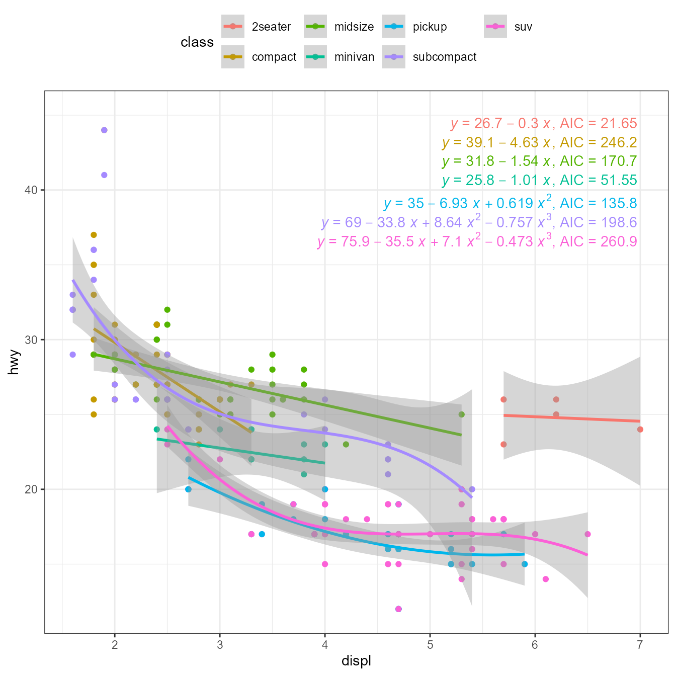
Note: Other approaches are possible because
additional arbitrary arguments can be passed by name to the method
function. Thus a more flexible approach would be to use R’s function
step() in the wrapper.
Functions that re-fit a fitted model
The examples in this section are for package ‘segmented’, however, a similar approach can be useful with any model fitting that involves calls to more than one function in sequence, such as computing starting values for a numerical method, or modifying the model fit object.
Segmented (‘segmented’)
Package ‘segmented’ implements methods for fitting models with change points. The location of the change points themselves are fitted with estimates and their standard deviations computed.
print(citation(package = "segmented", auto = TRUE), bibtex = FALSE)
#> To cite package 'segmented' in publications use:
#>
#>   Muggeo VMR (2026). _segmented: Regression Models with Break-Points /
#>   Change-Points Estimation (with Possibly Random Effects)_.
#>   doi:10.32614/CRAN.package.segmented
#>   <https://doi.org/10.32614/CRAN.package.segmented>. R package version
#>   2.2-1, <https://CRAN.R-project.org/package=segmented>.
library(segmented)The code here, is equivalent to that shown above based on model-fit
function segreg() also from package ‘segmented’. The
difference is that when using segmented() the fitting is
done in two steps. In this case there is no need to use this approach,
but it can be useful when segmentation is to be applied only to some
plot panels or applied conditionally in single panel plots. Another use
is when fitting segmented linear regressions based on model-fit
functions other than lm() or glm(). However,
in this second case, some of the necessary model-fit query functions can
be unavailable and may need to be defined by the user. There are also
model fit methods that do not compute or provide the estimates required
by the segmentation computations.
Package ‘segmented’ provides several specializations of method
segmented(). These methods are dispatched according to the
model fit object passed to parameter obj. As this package
provides all the expected query functions for the object
segmented() methods return, their use is not too difficult.
It is possible to write a wrapper function to pass as argument to
stat_poly_line() and stat_poly_eq() and in
addition, if used, construct the fitted equation labels within a call to
aes(). This function, that I named lm2segmented.lm, calls
first lm() and then calls segmented() with the
fitted model as argument. It accepts additional arguments that make it
possible to control the number and initial values of the knots. As in
the case of other model fit functions, models with multiple explanatory
variables are rarely used with ‘ggplot2’ stats.
lm2segmented.lm <-
  function(formula,
           data,
           seg.Z = ~ x, # explanatory variable used for segmentation
           psi = median(data$x), # starting value(s) for knot(s)
           npsi = 1, # number of knots if psi is not given
           fixed.psi = NULL, # breakpoint not to be modified by fitting
           control = seg.control(),
           ...) {
    obj <- lm(formula = formula, data = data, ...)
    segmented(obj = obj,
              seg.Z = seg.Z,
              psi = psi,
              npsi = npsi,
              fixed.psi = fixed.psi,
              control = control,
              model = TRUE,
              keep.class = FALSE)
  }
# using defaults, one breakpoint
ggplot(mpg, aes(displ, hwy)) +
  geom_point() +
  stat_poly_line(method = lm2segmented.lm)
ggplot(mpg, aes(displ, hwy)) +
  geom_hline(yintercept = 0, linetype = "dotted") +
  stat_fit_residuals(method = lm2segmented.lm) +
  labs(y = "Residuals")
# requesting two breakpoints with starting values
ggplot(mpg, aes(displ, hwy)) +
  geom_point() +
  stat_poly_line(method = lm2segmented.lm,
                 method.args = list(psi = c(3, 5)))
A more complex example with labels, assembled within the call to
aes(). In addition to the intercept and slope for the
leftmost segment, it returns the slope for each segment to the right of
the first one, but not their intercepts. As segment() fits
and returns the position of the knots, which are also returned by
stat_poly_eq() in ‘ggpmisc’ (>= 0.6.3). A label is added
with the knot position, and two regression equations, one for each
segment of the linear spline.
ggplot(mpg, aes(displ, hwy)) +
  geom_point() +
  stat_poly_eq(aes(label =
                     after_stat(
                       paste("italic(x)[cp]~`=`~",
                             round(knots[[1]][1], 2), "*\"; L: \"*y~`=`~",
                             round(b_0, 2), #"+",
                             round(b_1, 2), "~x*\"; R: \"*y~`=`~",
                             round(b_0 + knots[[1]][1] * (b_1 - b_2), 2), "+",
                             round(b_2, 2), "~x",
                             sep = ""))),
               parse = TRUE, output.type = "numeric",
               label.x = "right",
               formula = y ~ x,
               method = lm2segmented.lm) +
  stat_poly_eq(use_label("R2", "P", "AIC"),
               label.x = "right",
               label.y = 0.87,
               formula = y ~ x,
               method = lm2segmented.lm,
               method.args = list(psi = c(3, 5))) +
  stat_poly_line(method = lm2segmented.lm,
                 formula = y ~ x,)
Work-arounds
Some model-fit functions return objects for which no
predict() method exist. In such cases, as users we can
define such a method. More difficult situations can also be faced.
Errors in variables (‘refitME’)
In this section I show a situation I faced when trying to use package
‘refitME’. The functions exported by this package fail when called from
within a function, so they do not currently work if passed as an
argument for method. Below, a temporary work-around based
on a solution provided by the maintainer of ‘refitME’ is shown.
print(citation(package = "refitME", auto = TRUE), bibtex = FALSE)
#> To cite package 'refitME' in publications use:
#>
#>   Stoklosa J, Hwang W, Warton D (2025). _refitME: Measurement Error
#>   Modelling using MCEM_. doi:10.32614/CRAN.package.refitME
#>   <https://doi.org/10.32614/CRAN.package.refitME>. R package version
#>   1.3.1, <https://CRAN.R-project.org/package=refitME>.
library(refitME)As ‘refitME’ functions return a model fit object of the same class as
that received as input, a model fitted with lm() could be,
in principle, refit in a user-defined wrapper function as those above,
calling first lm() and re-fitting the obtained model with a
refitME::refitME() as shown in the code chunk below.
However, at the moment the functions in package ‘refitME’ fail when
called from within another function.
lm_EIV <- function(formula, data, ..., sigma.sq.u) {
  fm <- lm(formula = formula, data = data, ...)
  MCEMfit_glm(mod = fm, family = "gaussian", sigma.sq.u = sigma.sq.u)
}
After defining such a function, we could then use our function
lm_EIV() as the method.
ggplot(mpg, aes(displ, hwy)) +
   geom_point() +
   stat_poly_line(method = "lm_EIV", method.args = c(sigma.sq.u = 0)) +
   stat_poly_eq(method = "lm_EIV", method.args = c(sigma.sq.u = 0),
                mapping = use_label("eq"),
   label.x = "right") +
   theme(legend.position = "bottom") +
   facet_wrap(~class, ncol = 2)
However, it prints one warning like the one below for each call of the statistics.
Warning: Computation failed in `stat_poly_eq()`.
Caused by error in `names(new.dat)[c(1, which(names(mod$data) %in% names.w))] <- names(mod$data)[c(1, which(names(mod$data) %in% names.w))]`:
! replacement has length zero```
I have reported the problem through a GitHub issue to Jakub Stoklosa, the maintainer of ‘refitME’, and he is looking for a permanent solution. Meanwhile, he has provided a temporary fix that I copy below with a few small edits to the ggplot code. Many thanks to Jakub Stoklosa for his very fast answer!
rm(list = ls(pattern = "*"))

lm_EIV <- function(formula, data, ..., sigma.sq.u) {
  assign("my.data", value = data, envir = globalenv())
  fm <- lm(formula = formula, data = my.data, ...)
  fit <- refitME(fm, sigma.sq.u)

  fit$coefficients <- Re(fit$coefficients)
  fit$fitted.values <- Re(fit$fitted.values)
  fit$residuals <- Re(fit$residuals)
  fit$effects <- Re(fit$effects)
  fit$linear.predictors <- Re(fit$linear.predictors)
  fit$se <- Re(fit$se)

  if ("qr" %in% names(fit)) {
  fit$qr$qr <- Re(fit$qr$qr)
  fit$qr$qraux <- Re(fit$qr$qraux)
  }

  class(fit) <- c("lm_EIV", "lm")
  return(fit)
}

predict.lm_EIV <- function(object, newdata = NULL, ...) {
  preds <- NextMethod("predict", object, newdata = newdata, ...)

  if (is.numeric(preds)) {
    return(Re(preds))
  } else if (is.matrix(preds)) {
    return(Re(preds))
  } else {
    return(preds) # Leave unchanged if not numeric/matrix
  }
}
Here the limitation of ‘ggplot2’ and ‘ggpmisc’ in that the fit is
recomputed in each layer causes a further difficulty, as with most
algorithms using random numbers, the successive refits do not
necessarily produce the exact same results. In this case, the equation
and line are not matched, and the mismatch can be large for large values
of sigma.sq.u and low replication, especially in the
presence of outliers.
This is something that can most likely be fixed in ‘ggpmisc’ by
setting the seed of the RNG. To check that work-around is working as
expected, we set sigma.sq.u = 0 effectively using an OLS
approach and expecting values nearly identical as with
lm().
ggplot(mpg, aes(x = displ, y = hwy)) +
  geom_point() +
  stat_poly_line(aes(y = hwy),
                 method = "lm_EIV",
                 method.args = list(sigma.sq.u = 0)) +
  stat_poly_eq(aes(y = hwy,
                   label =
                     after_stat(
                       paste(eq.label, rr.label, sep = "~~"))),
               method = "lm_EIV",
               method.args = list(sigma.sq.u = 0),
               label.x = "right") +
  facet_wrap(~class, ncol = 2)
#> [1] 2
#> [1] 2
#> [1] 2
#> [1] 2
#> [1] 2
#> [1] 2
#> [1] 2
#> [1] 2
#> [1] 2
#> [1] 2
#> [1] 2
#> [1] 2
#> [1] 2
#> [1] 2
We do not know the measurement error for the measurement of
displ, the displacement volume of the engines. For this
example we make up a value: sigma.sq.u = 0.01 expecting
estimates different from above and with lm().
ggplot(mpg, aes(x = displ, y = hwy)) +
  geom_point() +
  stat_poly_line(aes(y = hwy),
                 method = "lm_EIV",
                 method.args = list(sigma.sq.u = 0.01)) +
  stat_poly_eq(aes(y = hwy,
                   label =
                     after_stat(
                       paste(eq.label, rr.label, sep = "~~"))),
               method = "lm_EIV",
               method.args = list(sigma.sq.u = 0.01),
               label.x = "right") +
  facet_wrap(~class, ncol = 2)
#> [1] 5
#> [1] 11
#> [1] 6
#> [1] 6
#> [1] 6
#> [1] 8
#> [1] 6
#> [1] 5
#> [1] 12
#> [1] 6
#> [1] 6
#> [1] 6
#> [1] 8
#> [1] 6
New data for prediction
Like in stat_smooth() from ‘ggplot2’, parameter
fullrange in stat_poly_line(),
stat_quant_line(), stat_quant_band() and
stat_ma_line() can be used to switch between prediction
based on the range of the explanatory variable data or based on the
limits of the scale of the corresponding aesthetic. Meanwhile,
n controls the number of equally spaced points at which the
prediction will be computed. In most use cases these two alternatives
are enough.
However, in some cases, finer control is useful. In plots with
facets, with major axis (MA) regression and possibly other model fits,
it can be useful to constrain the range of the prediction to that of the
response variable. Furthermore, in MA regression, the fitted line is the
same for y ~ x and x ~ y , thus simultaneously
restricting the range based on both x and y
seems logically preferable. Another case that cannot be automated with
stat_mooth() are predictions covering user-defined ranges
or for specific values of the explanatory variable.
In ‘ggpmisc’ (>= 1.0.0) the new limit.to parameter
provides the necessary control. The character strings
"x", "y", "xy" and
"none" make it possible for user to set which data range to
use as limit.
For these examples I expanded the x scale limits, so
that they are clearly broader than the default ones. These are rather
contrived examples demonstrating how fine control works.
The first example, with limit.to = "none" produces the
same plot as using fullrange = TRUE.
ggplot(subset(mpg, class == "suv"), aes(displ, hwy)) +
  geom_point() +
  stat_poly_line(limit.to = "none") +
  expand_limits(x = c(-2:10))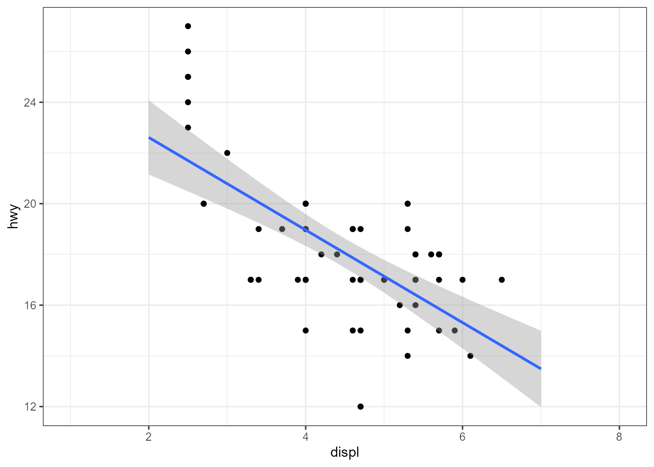
With limit.to = "y" the prediction is computed as in the
example above, but predicted values aoutside the range of y
are not passed to the geom, and, thus, not plotted.
ggplot(subset(mpg, class == "suv"), aes(displ, hwy)) +
  geom_point() +
  stat_poly_line(limit.to = "y") +
  expand_limits(x = c(-2:10))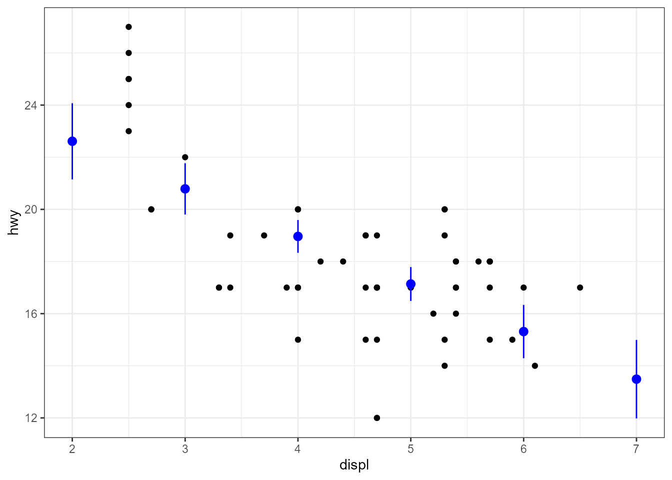
In addition to character strings as described above,
limit.to also accepts as argument a numeric vector to be
used as new data. This makes it possible to obtain a prediction for a
range that is neither that of the scale or that of the data. A use case
is when an unrestricted range could interfere with a plot
annotation.
ggplot(subset(mpg, class == "suv"), aes(displ, hwy)) +
  geom_point() +
  stat_poly_line(limit.to = seq(from = 2, to = 7, length.out = 80)) +
  expand_limits(x = c(1:8))
Although rarely useful when continuous variables are mapped to both
x and y, it is also possible to compute
predictions for discrete values of the explanatory variable. In this
example the predictions extend past the range of the data, and the range
of the limits of the scales are automatically extended for them to fit.
Instead of the default geom = "smooth",
geom = "pointrange" displays the individual
predictions.
ggplot(subset(mpg, class == "suv"), aes(displ, hwy)) +
  geom_point() +
  stat_poly_line(limit.to = 2:7,
                 geom = "pointrange",
                 colour = "blue")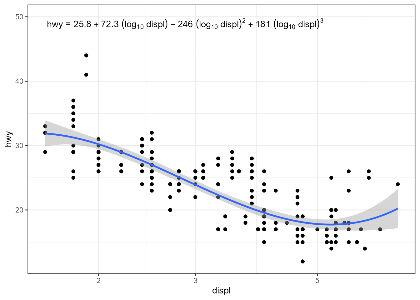
Transformations and eq.label
In ‘ggplot2’ setting transformations in x and y
scales results in statistics receiving transformed data as input. The
data “seen” by statistics is the same as if the transformation had been
applied within a call to aes(). However, the scales
automatically adjust breaks and tick labels to display the values in the
untransformed scale. When the transformation is applied in the model
formula definition, the transformation is applied later,
but still before the model is fit. all these cases, the model fit is
based on transformed values and thus the estimates refer to them. This
is why, a linear fit remains linear in spite of the transformations.
Only eq.label is affected by transformations in the
sense that the x and y in the default equation refer
to transformed values, rather than those shown in the tick labels of the
axes, i.e., the default model equation label is incorrect. The
correction to apply is to override the x and/or y
symbols in the equation label by an expression that includes the
transformation used. In these examples we fit polynomials by OLS using
lm(), the default method.
ggplot(mpg, aes(x = displ, y = hwy)) +
  geom_point() +
  stat_poly_line() +
  stat_poly_eq(mapping = use_label("eq", "R2", "n", "P"),
             eq.with.lhs = "log[10]~hwy~`=`~",
             eq.x.rhs = "~displ") +
  scale_y_log10() +
  expand_limits(y = 50)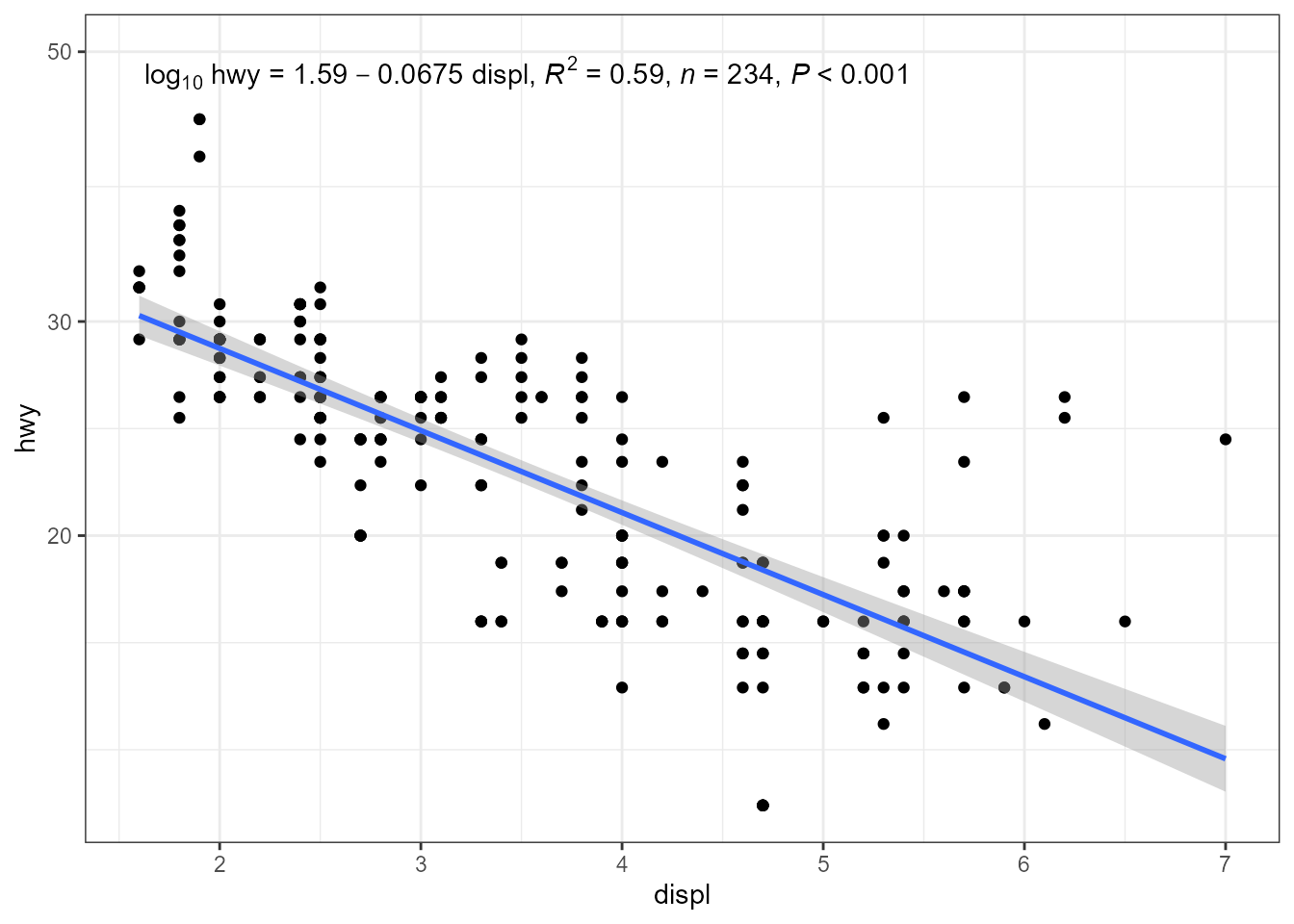
ggplot(mpg, aes(x = displ, y = hwy)) +
  geom_point() +
  stat_poly_line(formula = y ~ poly(x, 3, raw = TRUE)) +
  stat_poly_eq(mapping = use_label("eq"),
               formula = y ~ poly(x, 3, raw = TRUE),
               eq.with.lhs = "hwy~`=`~",
               eq.x.rhs = "~(log[10]~displ)") +
  scale_x_log10(name = "displ") +
  expand_limits(y = 50)