stat_spikes() tags or extracts rows in data containing local
y narrow maxima and/or minima with very steep shoulders. It makes it
possible to highlight and label spikes based on their x and/or
y coordinates. Orientations flipping as well as dates and times are
supported.
Usage
stat_spikes(
  mapping = NULL,
  data = NULL,
  geom = "point",
  position = "identity",
  ...,
  orientation = "x",
  height.threshold = 20,
  z.threshold = 7,
  k = 20,
  spike.direction = "both",
  label.fmt = NULL,
  x.label.fmt = label.fmt,
  y.label.fmt = NULL,
  extract.spikes = NULL,
  na.rm = FALSE,
  show.legend = FALSE,
  inherit.aes = TRUE
)
Arguments
- mapping
The aesthetic mapping, usually constructed with
aesoraes_. Only needs to be set at the layer level if you are overriding the plot defaults.- data
A layer specific dataset - only needed if you want to override the plot defaults.
- geom
The geometric object to use display the data
- position
The position adjustment to use for overlapping points on this layer
- ...
other arguments passed on to
layer. This can include aesthetics whose values you want to set, not map. Seelayerfor more details.- orientation
character The orientation of the layer can be set to either
"x", the default, or"y".- height.threshold
numeric The minimum height of spikes expressed relative to the median amplitude of the baseline local variation of
x.- z.threshold
numeric Modified local \(Z\) values larger than
z.thresholdare detected as boundaries of spikes.- k
integer width of median window used for smoothing; must be odd
- spike.direction
character One of
"up","down","both"or"skip", indicating which spikes are to be returned, if any.- label.fmt, x.label.fmt, y.label.fmt
character strings giving a format definition for construction of character strings labels with function
sprintffromxand/oryvalues.- extract.spikes
If
TRUEonly the rows containing spikes are returned. IfFALSEthe whole ofdatais returned but with labels set to""in rows not containing spikes. IfNULL, the default,TRUE, is used unless the argument passed togeomis"text_repel","label_repel"or"marquee_repel".- na.rm
a logical value indicating whether NA values should be stripped before the computation proceeds.
- show.legend
logical. Should this layer be included in the legends?
NA, the default, includes if any aesthetics are mapped.FALSEnever includes, andTRUEalways includes.- inherit.aes
If
FALSE, overrides the default aesthetics, rather than combining with them. This is most useful for helper functions that define both data and aesthetics and shouldn't inherit behaviour from the default plot specification, e.g.borders.
Value
A data frame with one row for each spike found in the data
extracted from the input data or all rows in data. Added columns
contain the labels.
Details
Spikes are detected based on a modified \(Z\) score calculated from the differenced spectrum. The \(Z\) threshold used should be adjusted to the characteristics of the input and desired sensitivity. The lower the threshold the more stringent the test becomes, with shorter spikes being detected.
The algorithm uses running differences to detect abrupt changes in value, compared to an estimate of the baseline variation of the differences, approximating a baseline \(Z\) from MAD and a baseline value from the median differences. Currently, a single estimate of MAD is used but running medians, when posisble, as baseline. This comparison detects running differences that are unusually large, in most cases signalling a transition between values near the baseline and far from it, in both directions.
Transitions into- and out of spikes are distinguished based on the median of the non-differenced values, as a descriptor of the data baseline. As for the median of the differences, a running median is used when possible.
This function thus detects the start and end of each spike, and distinguishes upward and downward spikes.
k is the width in number of observations of the window used for
running median smoothing to extract the baseline. A value several times the
width of the broader spike but narrow enough to track broader peaks needs
to be manually set in most cases.
With na.rm = TRUE, NA values are omitted before searching for
spikes and set to 0L in the returned vector.
If all spikes are guaranteed to be one observation-wide and either going up
or down from the baseline, it is possible to detect them based purely on
the z.threshold by passing height.threshold = NA and either
spike.direction = "up" or spike.direction = "down", which
ensures very fast computation.
Computed and copied variables in the returned data frame
- x
x-values at the spikes as numeric.
- y
y-values at the spikes as numeric.
- x.label
x-values at the spikes formatted as character.
- y.label
y-values at the spikes formatted as character.
- is.spike
integer vector of
0,1or-1.
Which variables are available for mapping?
Computed variables and
their names can vary depending on the method used to fit a model or
the output.type in use. They can also depend for a given
method on other arguments passed when fitting a model or extracting
estimates and other computed values. In many cases, when values are not
available, the variables are filled with NA values.
In the statistics returning formatted strings for use as annotations, a
message is issued by default in interactive R sessions, listing the short
names for available formatted labels as recognized by functions
use_label() and f_use_label(), except when
output.type = "numeric" is passed, in which case the names of all
variables accessible by after_stat() within a call to aes()
are listed. This default ("nicknames") can be changed by setting R
option "ggpmisc.stat.vars.message" to one of "names",
"colnames" or "none".
In the statistics that plot a prediction or more generally mainly return
numeric variables, a message is issued by default in interactive R
sessions, listing the names of all variables accessible by
after_stat() within a call to aes() with at least some
non-missing values. This default ("colnames") can be changed by
setting R option "ggpmisc.stat.vars.message" to "none".
To explore the whole returned data frame for a given input we suggest the
use of geom_debug().
Label positioning and formatting
stat_peaks(),
stat_valleys() and stat_spikes() work nicely together with
geoms geom_text_repel(), geom_label_repel(), and
geom_marquee_repel() from package ggrepel to
solve the problem of overlapping labels by displacing them. If using
geom_text(), discard overlapping labels using
check_overlap = TRUE.
By default the labels are character values ready to be ploted as plain
text, but with a suitable label.fmt argument, labels formatted as
plotmath expressions, markdown or LaTeX can be
created (e.g., containing Greek letters or super or subscripts, maths or
colour) can be generated for use with geoms from packages 'marquee',
'ggtext' and 'xdvir'.
The default is geom = "point" it is likely to work well in almost
any situation. The default aesthetics mappings set by these stats allow
their direct use with geom_text(), geom_label(),
geom_line(), geom_rug(), geom_hline() and
geom_vline() by just passing an argument to geom.
References
Whitaker, D. A.; Hayes, K. (2018) A simple algorithm for despiking Raman spectra. Chemometrics and Intelligent Laboratory Systems, 179, 82-84. doi:10.1016/j.chemolab.2018.06.009 .
See also
find_peaks() for functions suitable for broader
peaks and valleys.
Aesthetics
stat_spikes() understands the following aesthetics. Required aesthetics are displayed in bold and defaults are displayed for optional aesthetics:
| • | x | |
| • | y | |
| • | group | → inferred |
| • | label | → after_stat(x.label) |
| • | xintercept | → after_stat(x) |
| • | yintercept | → after_stat(y) |
Learn more about setting these aesthetics in vignette("ggplot2-specs").
Examples
# lynx and Nile are time.series objects recognized by
# ggpp::ggplot.ts() and converted on-the-fly with a default mapping
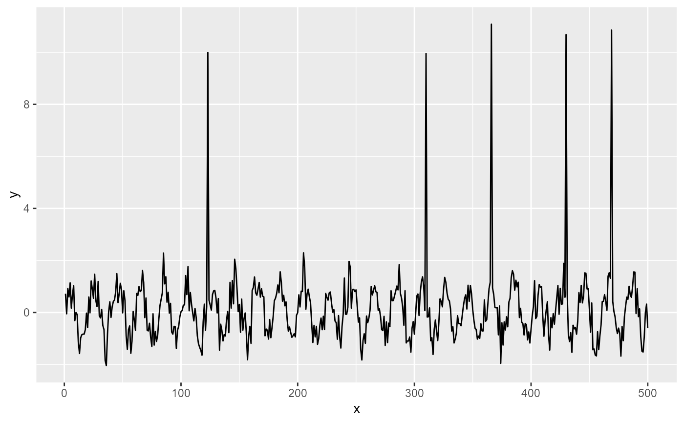
n = 500
set.seed(45678)
my.data <- data.frame(x = 1:n,
y = rep(sin((0:19)/20 * 2 * pi), n / 20) +
stats::rnorm(n, sd = 0.5))
selector <- sample(seq_len(n), 5)
my.data$y[selector] <- my.data$y[selector] + 10
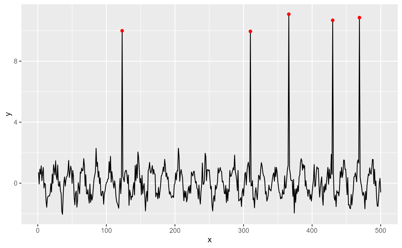
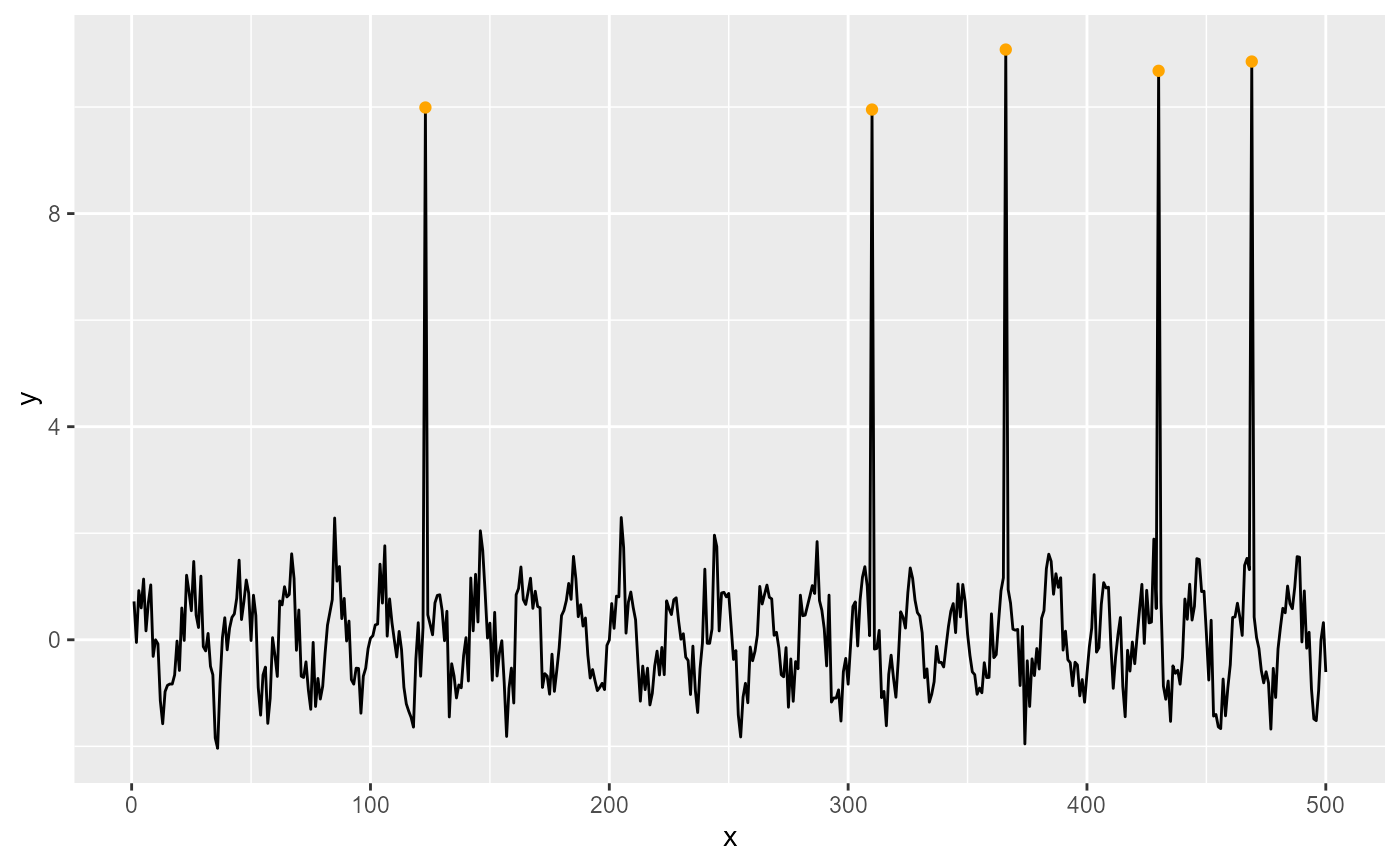
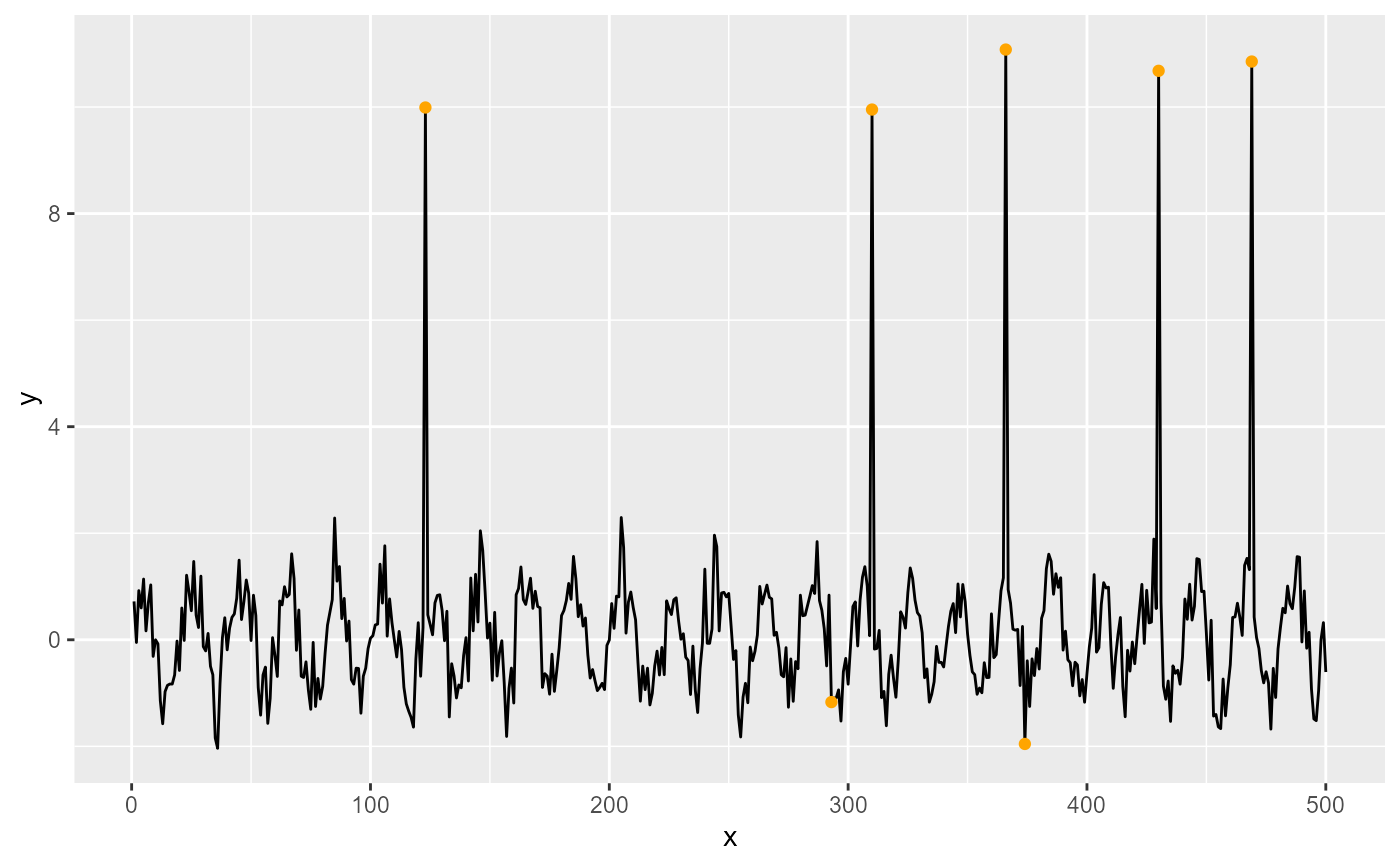
ggplot(my.data, aes(x, y)) +
geom_line() +
stat_spikes(colour = "orange")
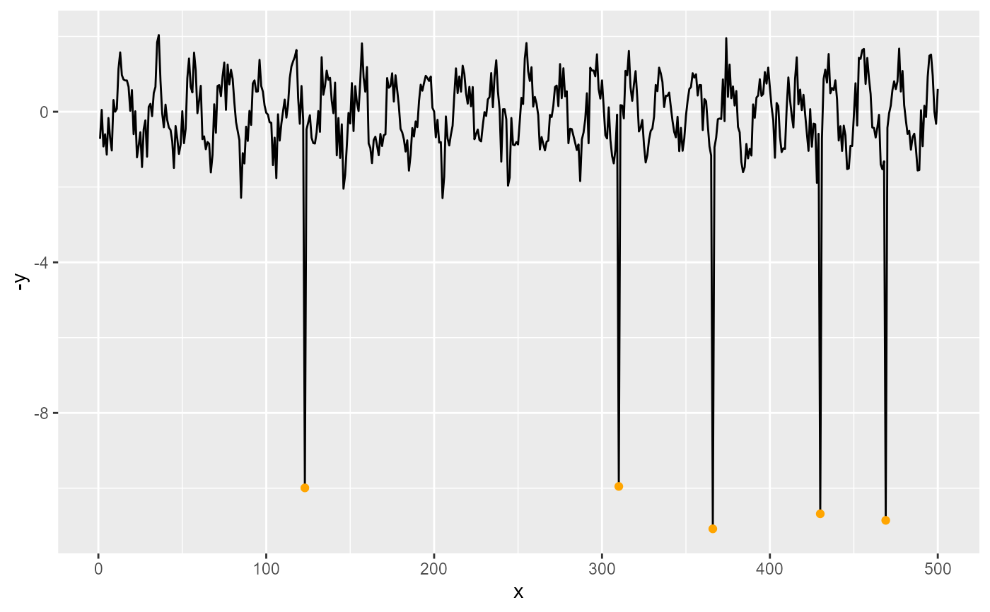
 ggplot(my.data, aes(x, -y)) +
geom_line() +
stat_spikes(colour = "orange")
ggplot(my.data, aes(x, -y)) +
geom_line() +
stat_spikes(colour = "orange")
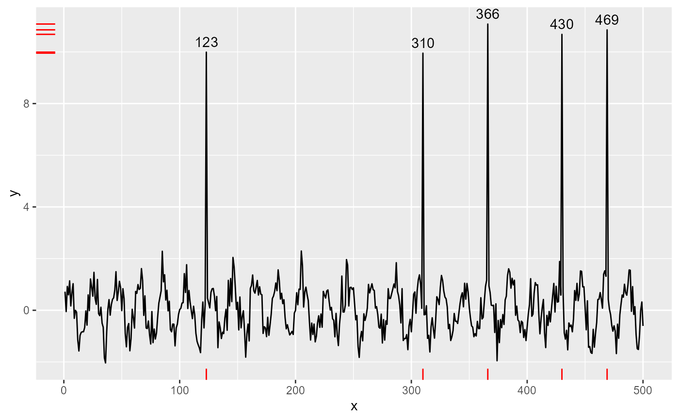
 ggplot(my.data, aes(x, y)) +
geom_line() +
stat_spikes(geom = "text", vjust = -0.5) +
stat_spikes(geom = "rug", colour = "red")
ggplot(my.data, aes(x, y)) +
geom_line() +
stat_spikes(geom = "text", vjust = -0.5) +
stat_spikes(geom = "rug", colour = "red")
 ggplot(my.data, aes(x, y)) +
geom_line() +
stat_spikes(colour = "red", spike.direction = "up") +
stat_spikes(colour = "blue", spike.direction = "down")
ggplot(my.data, aes(x, y)) +
geom_line() +
stat_spikes(colour = "red", spike.direction = "up") +
stat_spikes(colour = "blue", spike.direction = "down")
 ggplot(my.data, aes(x, y)) +
geom_line() +
stat_spikes(colour = "red", spike.direction = "up")
ggplot(my.data, aes(x, y)) +
geom_line() +
stat_spikes(colour = "red", spike.direction = "up")
 ggplot(my.data, aes(x, y)) +
geom_line() +
stat_spikes(colour = "blue", spike.direction = "down")
ggplot(my.data, aes(x, y)) +
geom_line() +
stat_spikes(colour = "blue", spike.direction = "down")
 ggplot(my.data, aes(x, y)) +
geom_line() +
stat_spikes(z.threshold = 2, colour = "orange")
ggplot(my.data, aes(x, y)) +
geom_line() +
stat_spikes(z.threshold = 2, colour = "orange")
 ggplot(my.data, aes(x, y)) +
geom_line() +
stat_spikes(z.threshold = 20, colour = "orange")
ggplot(my.data, aes(x, y)) +
geom_line() +
stat_spikes(z.threshold = 20, colour = "orange")
 ggplot(my.data, aes(x, y)) +
geom_line() +
stat_spikes(colour = "red",
spike.direction = "up",
height.threshold = NA)
ggplot(my.data, aes(x, y)) +
geom_line() +
stat_spikes(colour = "red",
spike.direction = "up",
height.threshold = NA)