Multiple comparisons

Aims of ‘ggpmisc’ and caveats

Package ‘ggpmisc’ makes it easier to add to plots created using ‘ggplot2’ annotations based on fitted models and other statistics. It does this by wrapping existing model fit and other functions. The same annotations can be produced by calling the model fit functions, extracting the desired estimates and adding them to plots. There are two advantages in wrapping these functions in an extension to package ‘ggplot2’: 1) we ensure the coupling of graphical elements and the annotations by building all elements of the plot using the same data and a consistent grammar and 2) we make it easier to annotate plots to the casual user of R, already familiar with the grammar of graphics.

To avoid confusion it is good to make clear what may seem obvious to some: if no plot is needed, then there is no reason to use this package. The values shown as annotations are not computed by ‘ggpmisc’ but instead by the usual model-fit and statistical functions from R and R packages. The same is true for model predictions, residuals, etc. that some of the functions in ‘ggpmisc’ display as lines, segments, or other graphical elements.

It is also important to remember that in most cases data analysis including exploratory and other stages should take place before annotated plots for publication are produced. Even though data analysis can benefit from combined numerical and graphical representation of the results, the use I envision for ‘ggpmisc’ is mainly for the production of plots for publication or communication. In either case, whether used for analysis or communication, it is crucial that users cite and refer both to ‘ggpmisc’ and to the underlying R and R packages when publishing plots created with functions and methods from ‘ggpmisc’.

print(citation(package = "ggpmisc", auto = TRUE), bibtex = FALSE)
#> To cite package 'ggpmisc' in publications use:
#> 
#>   Aphalo P (2026). _ggpmisc: Miscellaneous Extensions to 'ggplot2'_. R
#>   package version 1.0.0.9000,
#>   <https://docs.r4photobiology.info/ggpmisc/>.

In experimental designs with more than two groups or treatments, we face the problem that testing every possible pair for significant difference, includes a test of the smallest vs. the largest observed value. This means that the probability of at least one pair being significant is no longer the one computed in a t-test or LSD (least significant difference). We need to distinguish the probability of making the wrong decision in an individual comparison (comparison-wise) from that for the experiment as a whole (experiment-wise, the number of wrong decisions per experiment).

There are different approaches, that can be grouped into methods that attempt to control the experiment-wise probability of false positive outcomes to a given P-level, such as 0.05 (adjusted P-values), and those that attempt to control the false discovery rate (FDR), that can be thought of as the proportion of the positive outcomes that are false positives. There are variations in both approaches, varying in power and conservativeness.

A correction needs to be applied to P-values or LSD. Different methods are available for this. Methods differ in their assumptions and difficulty of computation. Tukey’s HSD (honestly significant difference) and the Bonferroni correction are well known approaches. Bonferroni’s method is a “quick and dirty” calculation but nowadays not recommended as it applies an unnecessarily strong correction.

Dunnet contrasts test all treatments individually against a control condition. Tukey contrasts targets the case of testing all possible pairs. It is also possible to set-up contrasts of interest individually, or testing for other differences, such as basing them on the average of related treatments.

In general, one should test for significant differences only those contrasts selected a priori as of interest. The fewer the pairs tested for significance, the smaller a correction needs to be applied, thus increasing the power of the test for the cases of interest. Of course, for validity, which tests are of interest should be decided independently of the data.

Multiple comparisons are frequently applied as post-hoc tests (after a different test of significance with a broader scope). As post-hoc tests, they are seen as a way of investigating the source of an overall significant difference, and multiple comparisons are applied only if the main effect of the factor is in itself significant and the additional contrasts skipped otherwise. In other cases multiple comparisons can be the primary statistical test addressing the research hypotheses. Both approaches are valid as long as the hypotheses have been set independently of the data being used in the test.

Plot annotations for multiple comparison tests

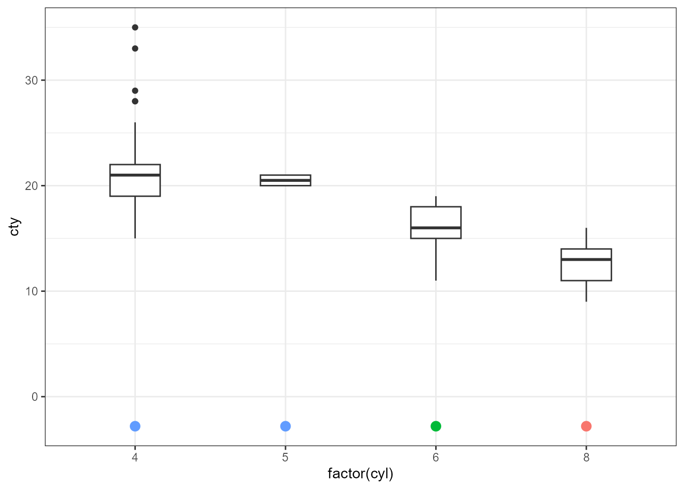
The letter labels and labelled segments used to highlight pairwise comparisons are a special case as they behave as data labels along the axis onto which an explanatory factor has been mapped, usually x, but frequently as annotations along the axis onto which a continuous numeric variable has been mapped, usually y.

Layer function stat_multcomp() first fits a model (a linear model by default) followed by a multiple comparisons’ test with a user-controlled adjustment to the P-values. The implementation makes use of function glht() from package multcomp making available all the methods it supports for the adjustment of P-values for multiple comparisons. Currently, stat_multcomp() only implements pairwise contrasts, as in this case there are well established approaches to plot annotations. By passing a numeric matrix as argument arbitrary sets of pairwise contrasts can be specified. _Contrasts that are not pairwise, i.e., that involve more than two levels of a factor, are not yet supported.

The returned value and default geometry depend on the type of label, that can be either bars (connecting segments) labelled with P-values or other parameters, or letters.

Examples

Package ggpmisc imports and re-exports all definitions from ggpp as well as from ggplot2, so it is enough to attach explicitly package ggpmisc . All three packages are available through CRAN.

library(ggpmisc)
theme_set(theme_bw())

Using default labels

Tukey’s method for all pairwise contrasts using honestly significant differences, while adjusting the size and position of the labels.

ggplot(mpg, aes(factor(cyl), cty)) +
  stat_summary(fun.data = mean_cl_normal, 
               colour = "red") +
  stat_multcomp(label.y = 12, 
                size = 2.75, 
                vstep = 0.05) +
  expand_limits(y = 0)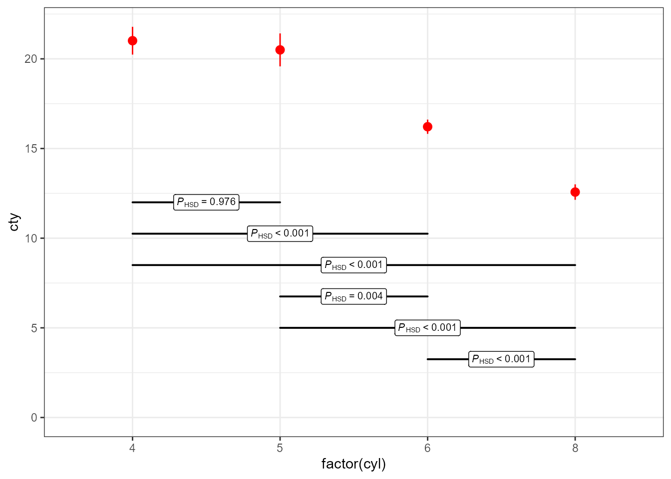

Using Holm’s method to adjust P-values.

ggplot(mpg, aes(factor(cyl), cty)) +
  stat_summary(fun.data = mean_cl_normal, colour = "red") +
  stat_multcomp(p.adjust.method = "holm",
                label.y = 12, 
                size = 2.75, 
                vstep = 0.05) +
  expand_limits(y = 0)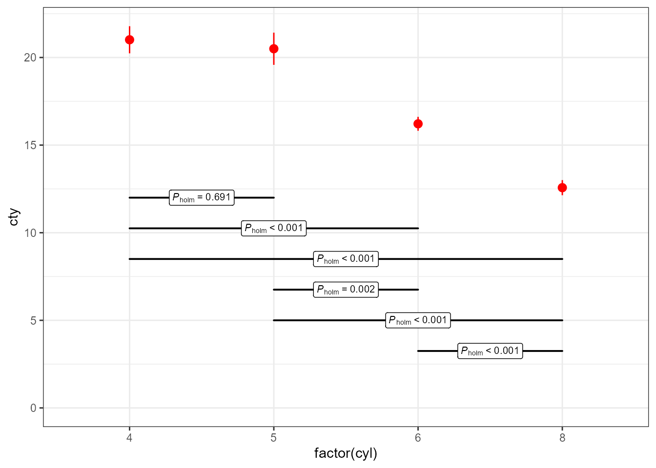

Dunnet’s method for comparison of each treatment against a control, assumed to be the first level of the factor.

ggplot(mpg, aes(factor(cyl), cty)) +
  stat_summary(fun = mean, geom = "col", width = 0.5) +
  stat_summary(fun.data = mean_cl_normal, colour = "red") +
  stat_multcomp(label.y = 25, 
                size = 2.75,
                contrasts = "Dunnet")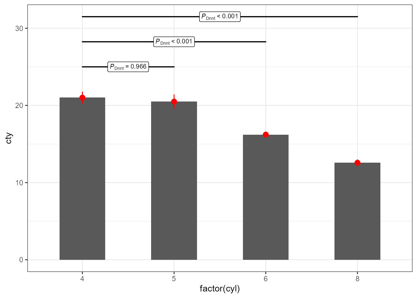

A staircase of pairwise contrasts with P-values adjusted using Holm’s method.

ggplot(mpg, aes(factor(cyl), cty)) +
  stat_summary(fun = mean, geom = "col", width = 0.5) +
  stat_summary(fun.data = mean_cl_normal, colour = "red") +
  stat_multcomp(label.y = c(18, 23, 24),
                size = 2.75,
                contrasts = rbind(c(0, 0, -1, 1),
                                  c(0, -1, 1, 0),
                                  c(-1, 1, 0, 0)))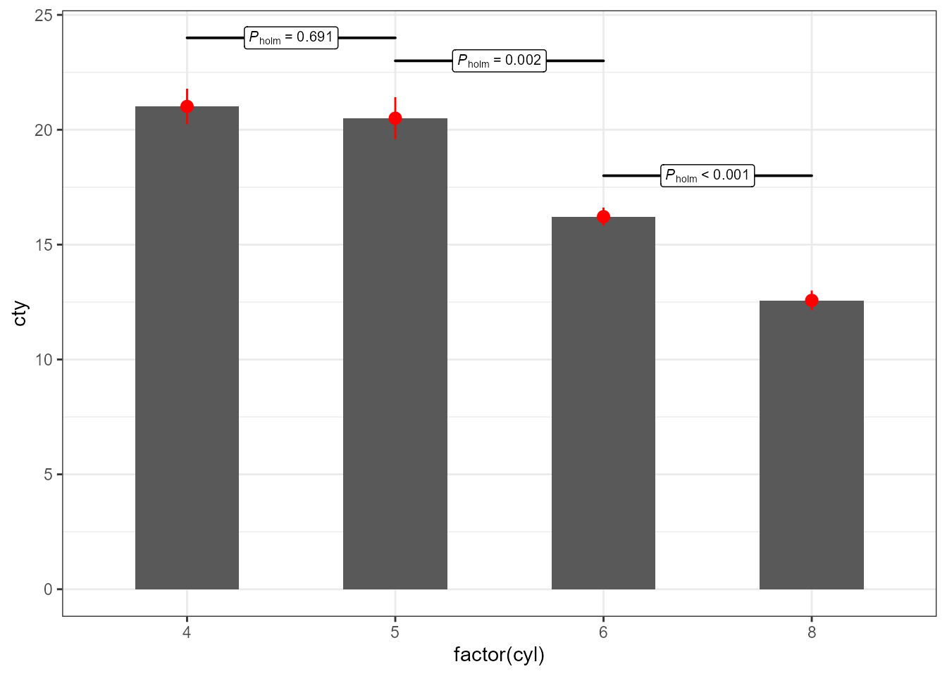

Tukey’s pairwise contrasts using defaults except for the position of the lowermost bar.

ggplot(mpg, aes(factor(cyl), cty)) +
  stat_summary(fun = mean, geom = "col", width = 0.5) +
  stat_summary(fun.data = mean_cl_normal, colour = "red") +
  stat_multcomp(size = 2.5, label.y = 25)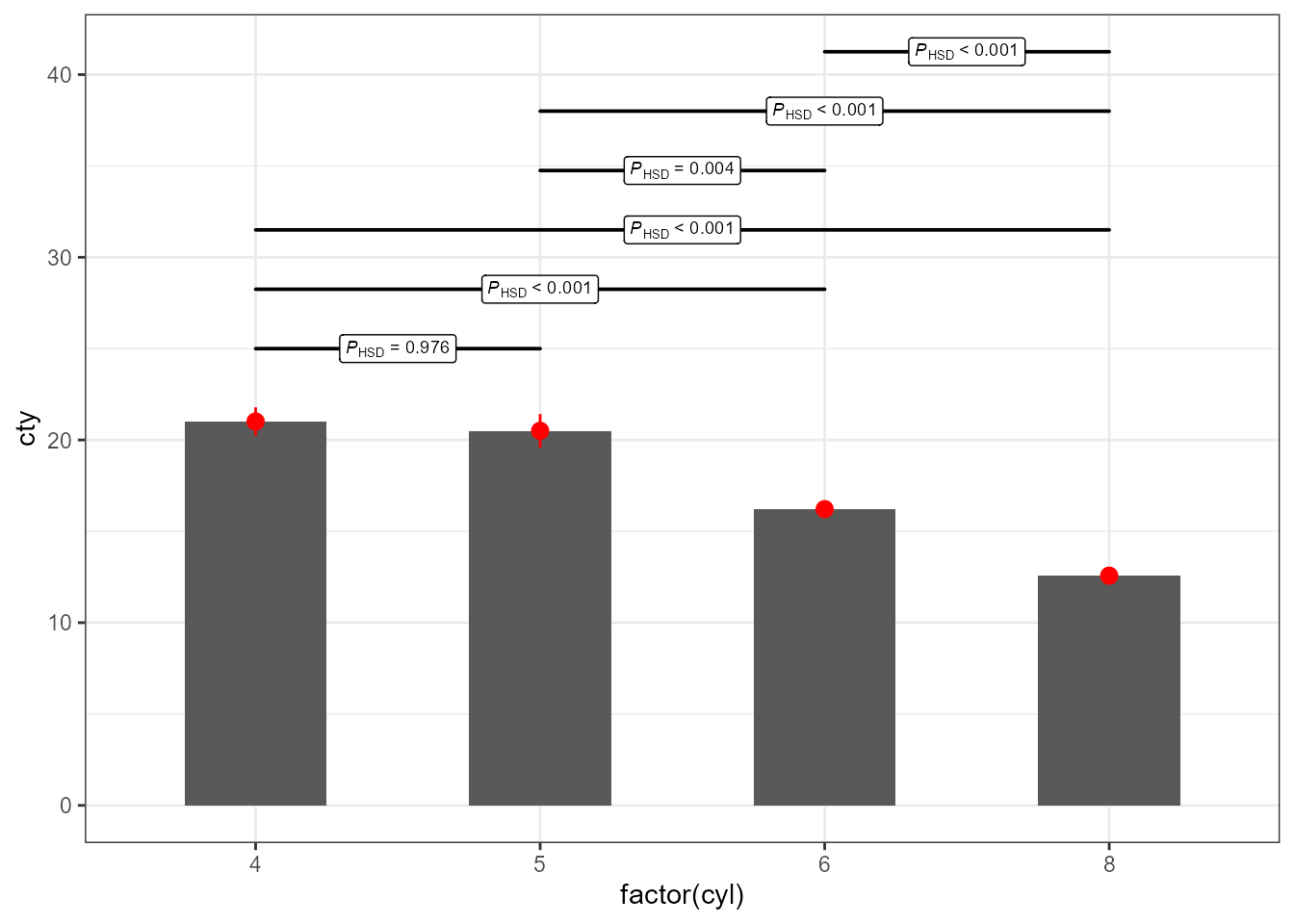

Tukey’s pairwise contrasts using defaults and shown with letters.

ggplot(mpg, aes(factor(cyl), cty)) +
  stat_summary(fun = mean, geom = "col", width = 0.5) +
  stat_summary(fun.data = mean_cl_normal, colour = "red") +
  stat_multcomp(label.y = -1, 
                label.type = "letters")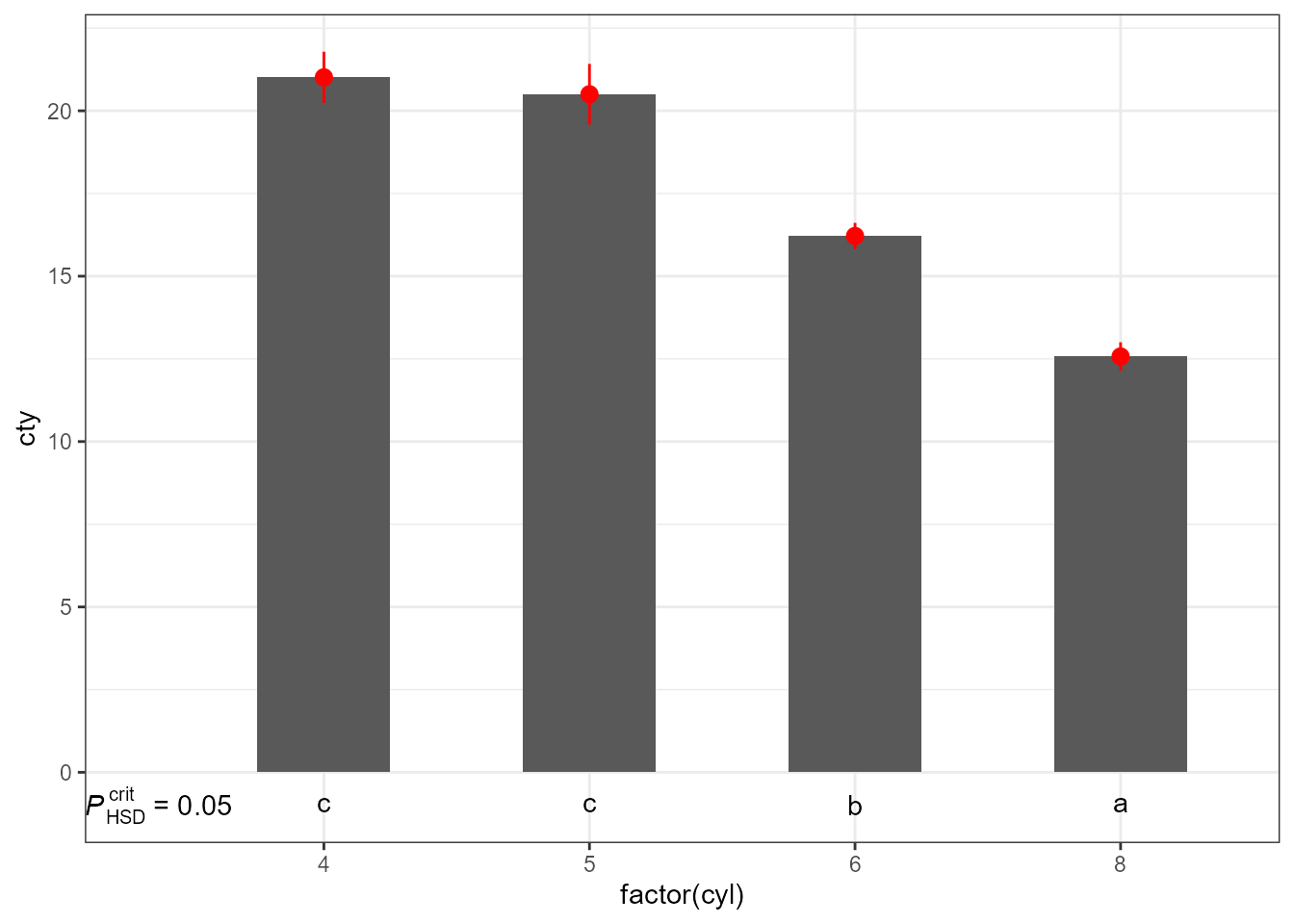

ggplot(mpg, aes(factor(cyl), cty)) +
  stat_summary(fun = mean, geom = "col", width = 0.5) +
  stat_summary(fun.data = mean_cl_normal, colour = "red") +
  stat_multcomp(colour = "white", 
                label.type = "letters",
                adj.method.tag = 0)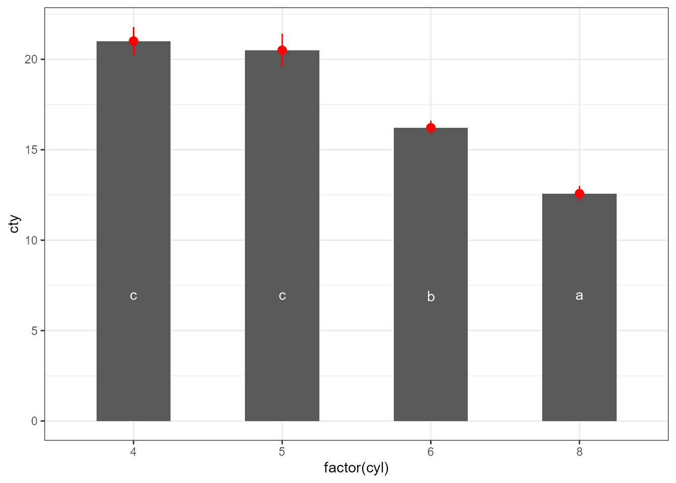

ggplot(mpg, aes(factor(cyl), cty)) +
  stat_multcomp(size = 2.75) +
  stat_boxplot(width = 1/3)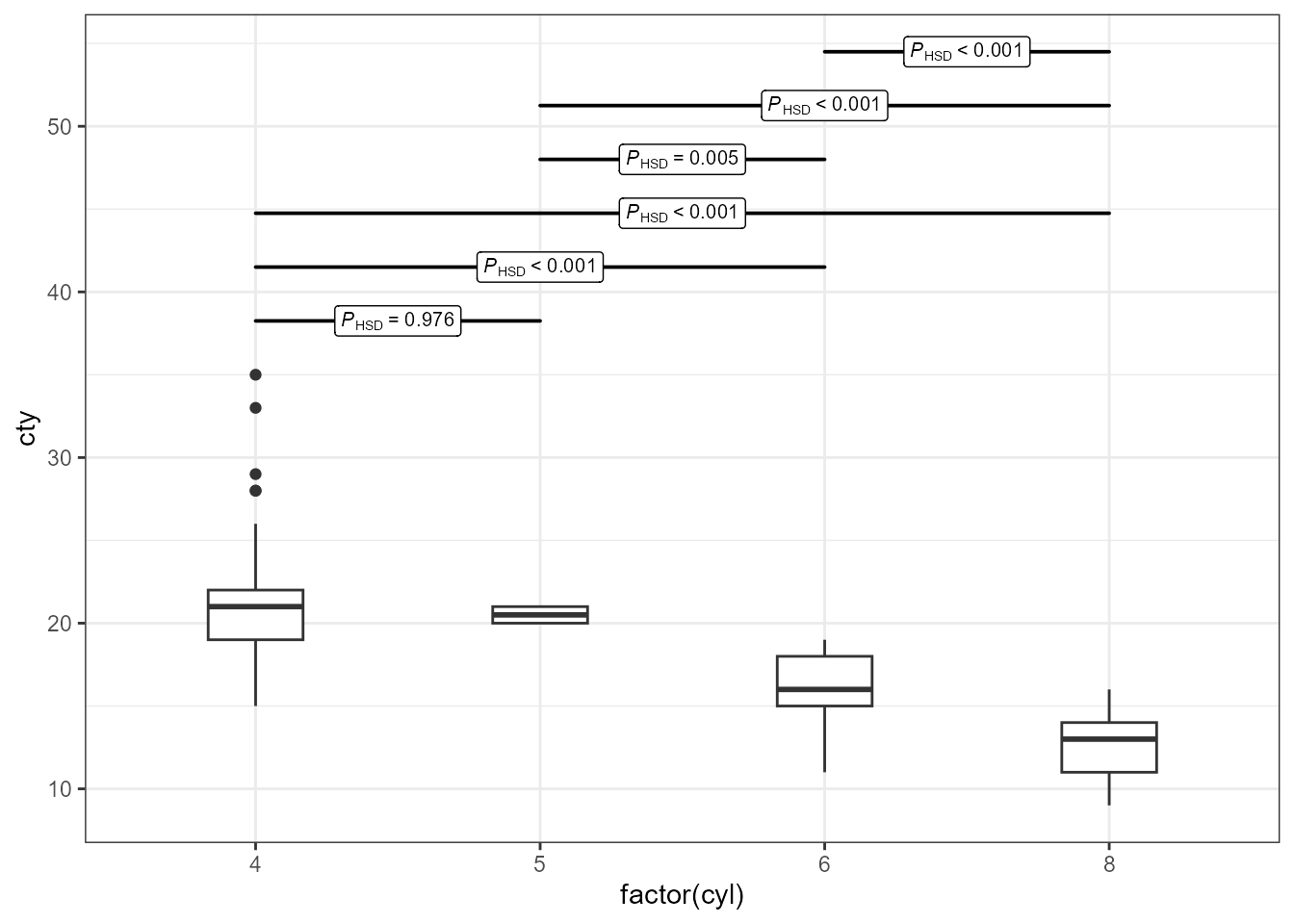

ggplot(mpg, aes(factor(cyl), cty)) +
  stat_multcomp(size = 2.85,
                label.y = 11,
                geom = "text_pairwise",
                vstep = 0.07,
                p.digits = 2,
                contrasts = "Dunnet") +
  stat_boxplot(width = 1/3) +
  expand_limits(y = 0)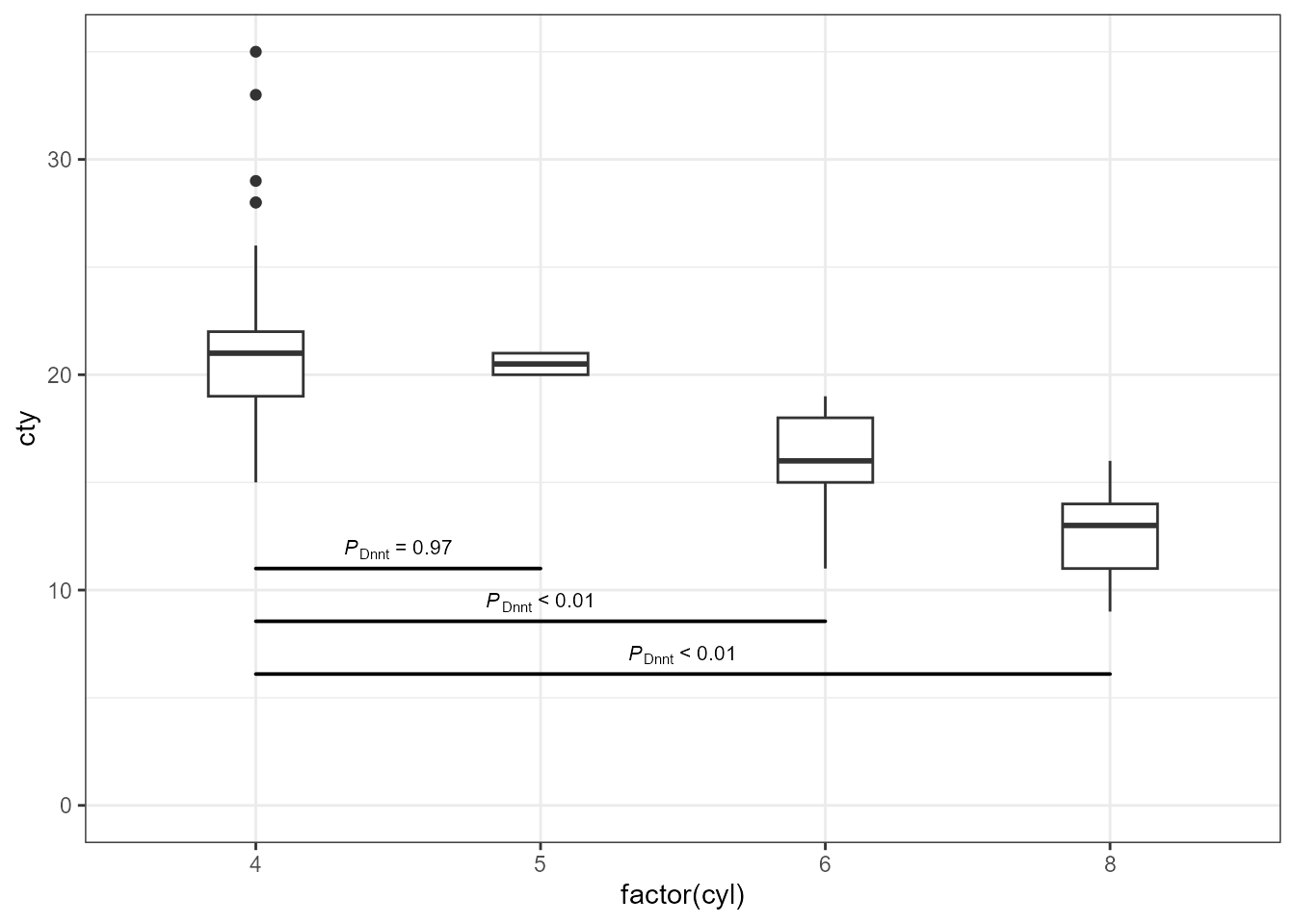

ggplot(mpg, aes(factor(cyl), cty)) +
  stat_multcomp(label.type = "letters",
                geom = "label",
                size = 2.75) +
  stat_boxplot(width = 1/3)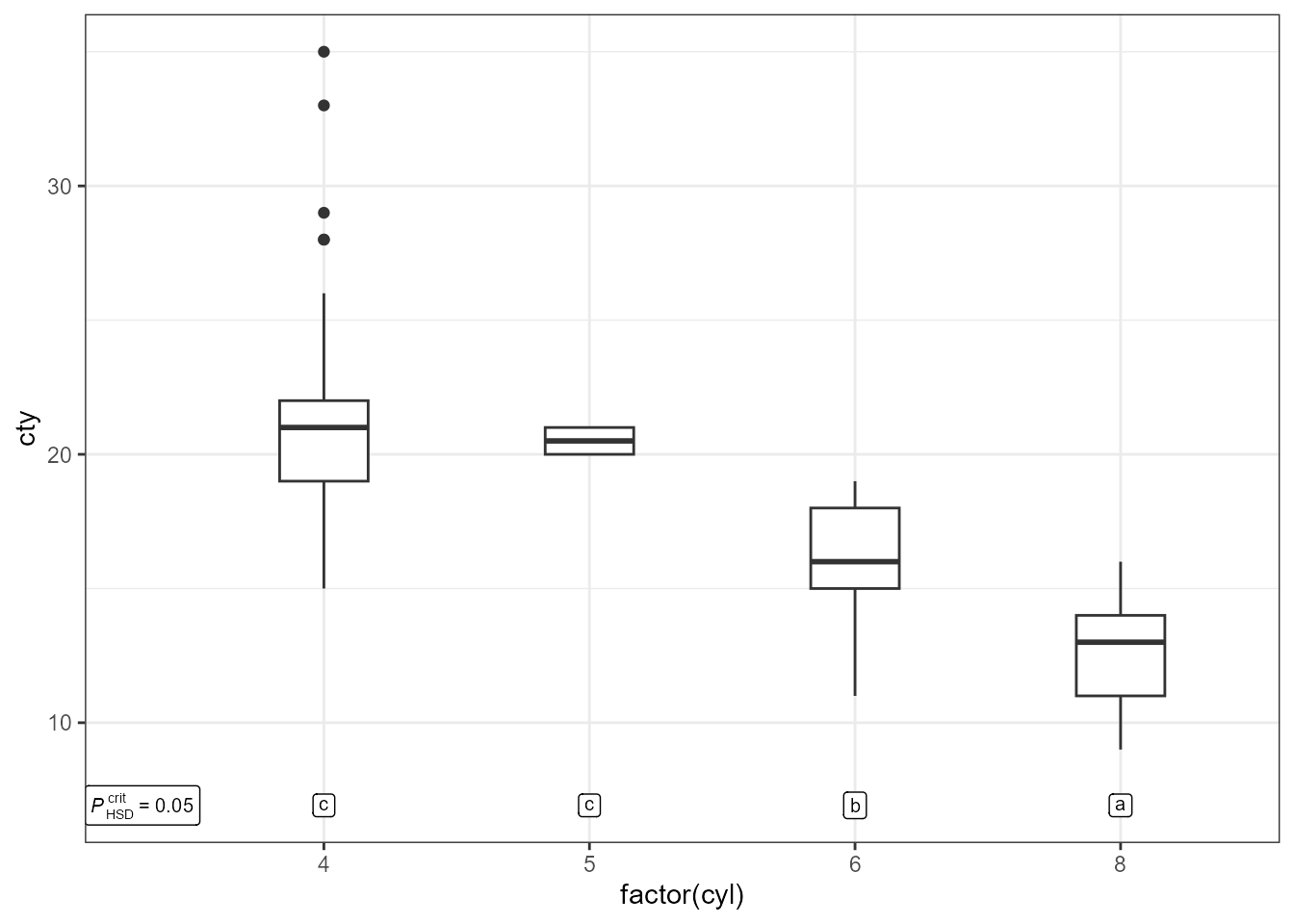

Numeric P-values shown for Dunnet contrasts.

ggplot(mpg, aes(factor(cyl), cty)) +
  stat_summary(fun = mean, geom = "col", width = 0.5) +
  stat_summary(fun.data = mean_cl_normal, colour = "red") +
  stat_multcomp(aes(x = stage(start = factor(cyl), 
                              after_stat = xmax)),
                geom = "text",
                label.y = -1, 
                vstep = 0,
                size = 3,
                contrasts = "Dunnet")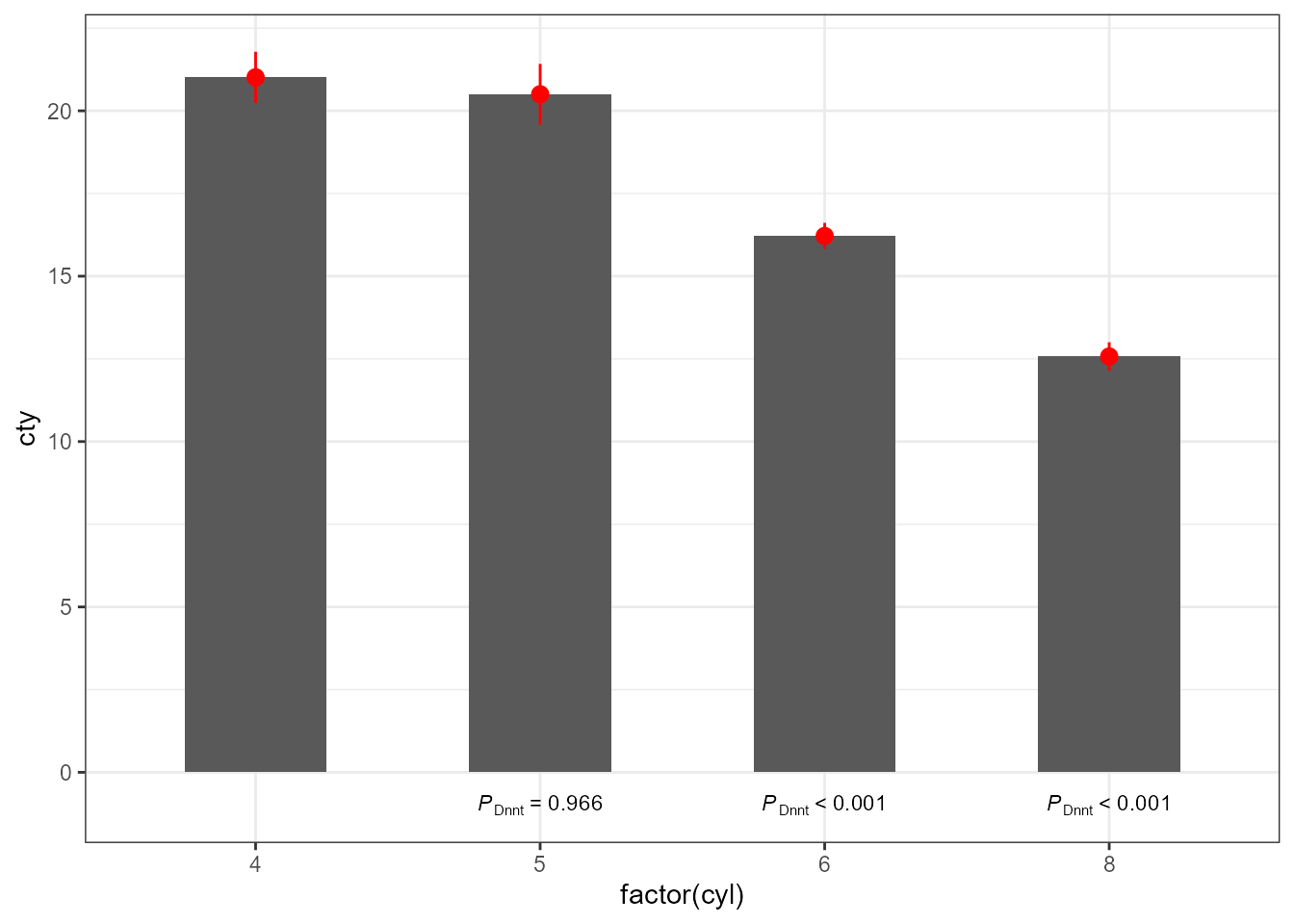

Using pre-built labels other than default

ggplot(mpg, aes(factor(cyl), cty)) +
  stat_multcomp(use_label(c("delta", "P")),
                size = 2.75,
                label.y = 11,
                vstep = 0.08,
                p.digits = 2,
                contrasts = "Dunnet") +
  stat_boxplot(width = 1/3) +
  expand_limits(y = 0)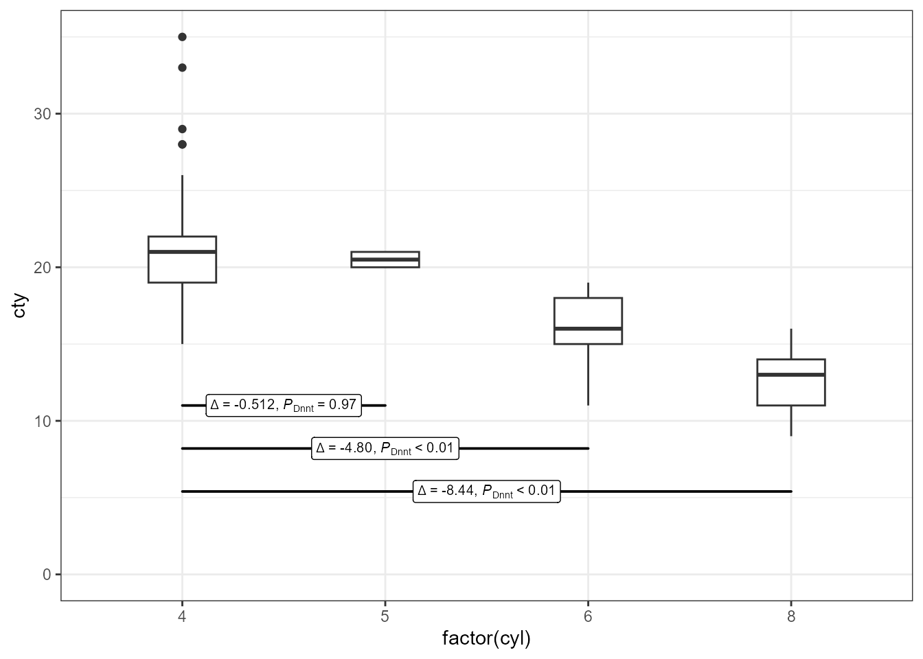

ggplot(mpg, aes(factor(cyl), cty)) +
  stat_multcomp(use_label(c("t", "P")),
                          size = 2.75,
                label.y = 11,
                vstep = 0.08,
                contrasts = "Dunnet") +
  stat_boxplot(width = 1/3) +
  expand_limits(y = 0)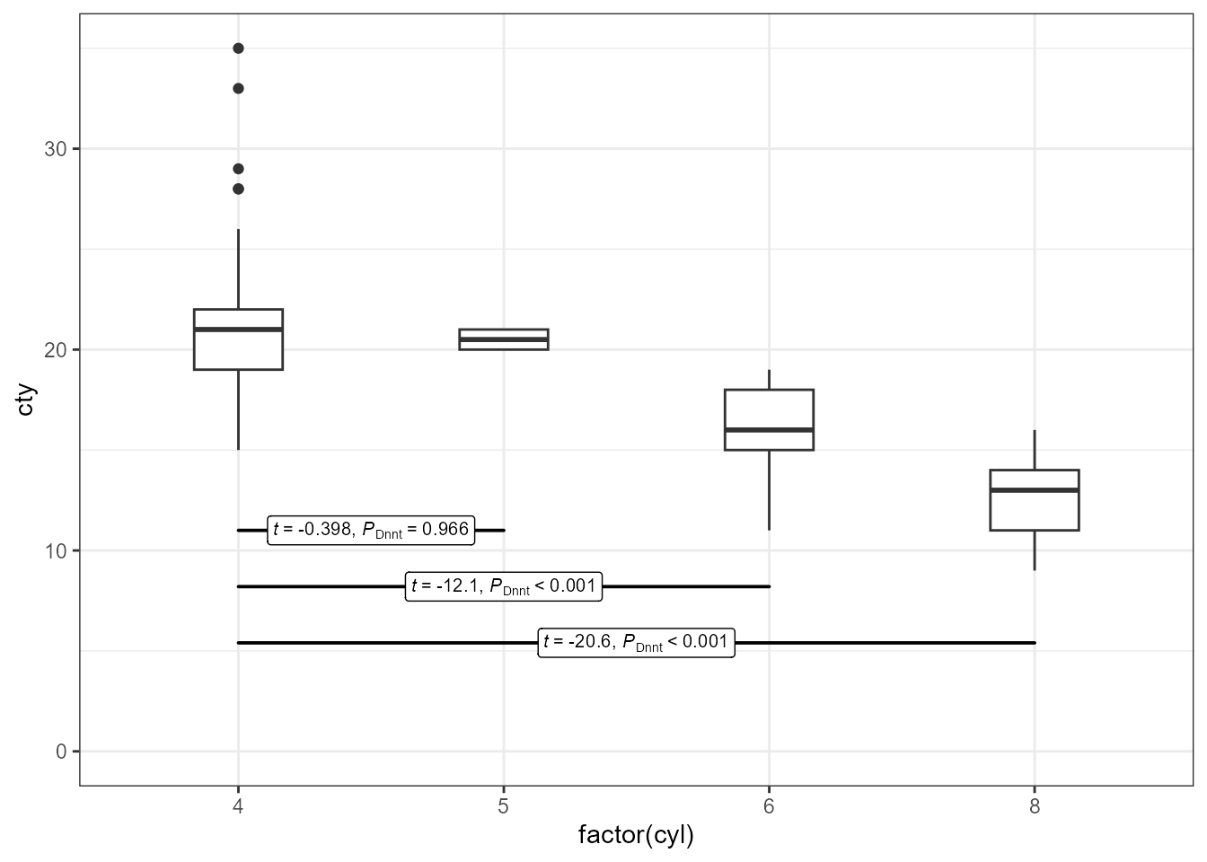

ggplot(mpg, aes(factor(cyl), cty)) +
  stat_summary(fun = mean, geom = "col", width = 0.5) +
  stat_summary(fun.data = mean_cl_normal, colour = "red") +
  stat_multcomp(aes(x = stage(start = factor(cyl), after_stat = xmax),
                    label = after_stat(stars.label)),
                geom = "text",
                label.y = -1,
                vstep = 0,
                contrasts = "Dunnet")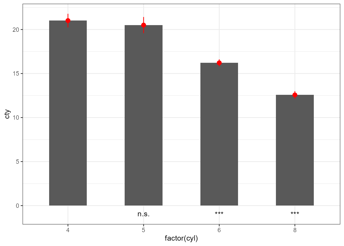

Using other aesthetics than the default

ggplot(mpg, aes(factor(cyl), cty)) +
  stat_multcomp(aes(colour = after_stat(p.value) < 0.05),
                size = 2.75,
                label.y = 11,
                vstep = 0.08,
                p.digits = 2,
                contrasts = "Dunnet") +
  stat_boxplot(width = 1/3) +
  scale_colour_manual(values = c("grey50", "blue")) +
  expand_limits(y = 0)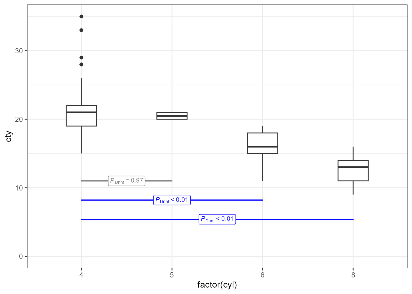

ggplot(mpg, aes(factor(cyl), cty)) +
  stat_multcomp(aes(fill = after_stat(p.value) < 0.05),
                size = 2.75,
                label.y = 11,
                vstep = 0.08,
                p.digits = 2,
                contrasts = "Dunnet") +
  stat_boxplot(width = 1/3) +
  scale_fill_manual(values = c("grey90", "lightblue")) +
  expand_limits(y = 0)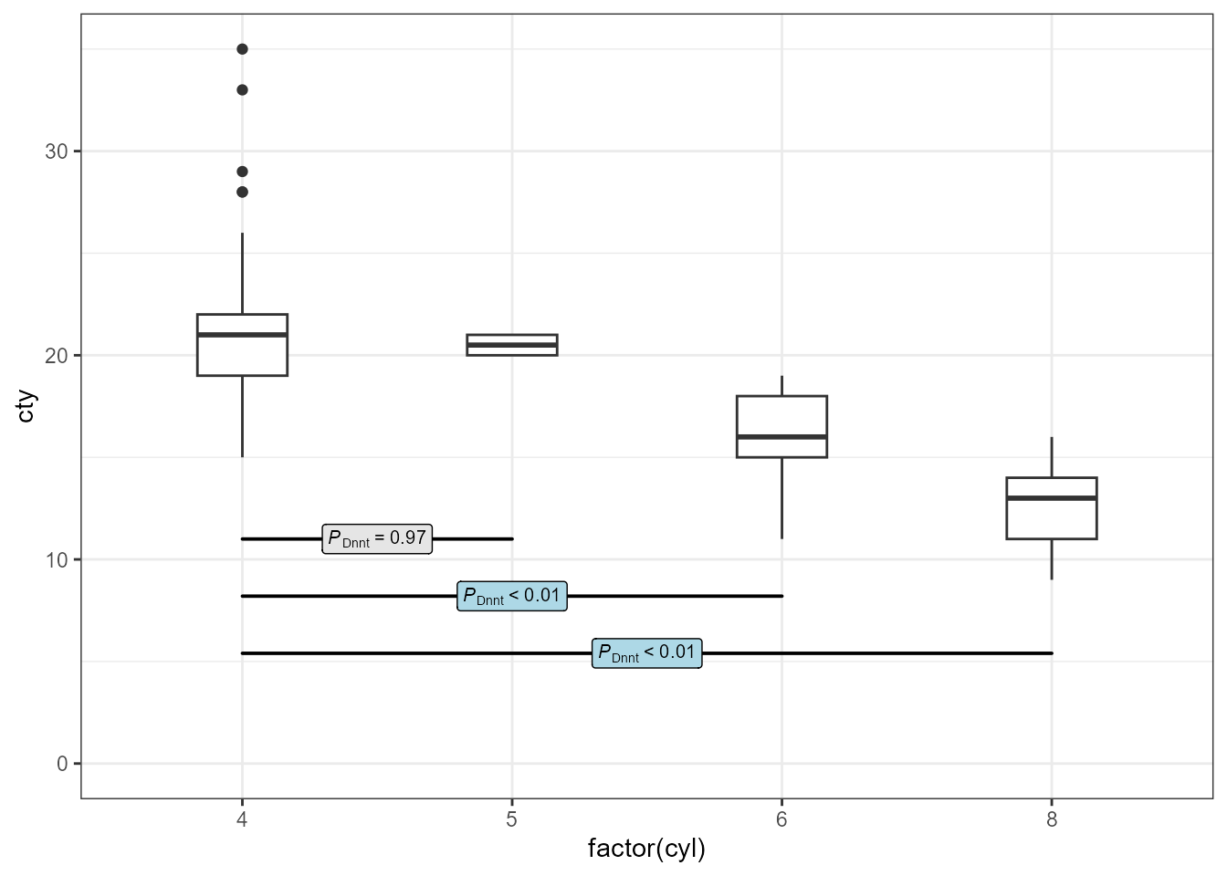

ggplot(mpg, aes(factor(cyl), cty)) +
  stat_multcomp(aes(colour = factor(after_stat(letters.label))),
                label.type = "letters",
                size = 4) +
  stat_boxplot(width = 1/3) +
  expand_limits(y = 0)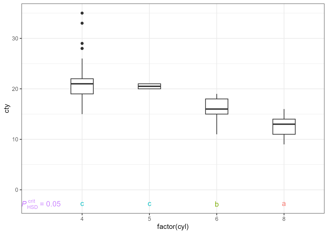

ggplot(mpg, aes(factor(cyl), cty)) +
  stat_multcomp(aes(colour = factor(after_stat(letters.label))),
                label.type = "letters",
                geom = "point",
                size = 3,
                adj.method.tag = 0) +
  stat_boxplot(width = 1/3) +
  expand_limits(y = 0)

Multiple comparisons

‘ggpmisc’ 1.0.0.9000

Pedro J. Aphalo

2026-07-08

Aims of ‘ggpmisc’ and caveats