Comparison of output types
‘ggpmisc’ 1.0.0.9000
Pedro J. Aphalo
2026-07-08
Source:vignettes/articles/output-types.Rmd
output-types.RmdAims of ‘ggpmisc’ and caveats
Package ‘ggpmisc’ makes it easier to add to plots created using ‘ggplot2’ annotations based on fitted models and other statistics. It does this by wrapping existing model fit and other functions. The same annotations can be produced by calling the model fit functions, extracting the desired estimates and adding them to plots. There are two advantages in wrapping these functions in an extension to package ‘ggplot2’: 1) we ensure the coupling of graphical elements and the annotations by building all elements of the plot using the same data and a consistent grammar and 2) we make it easier to annotate plots to the casual user of R, already familiar with the grammar of graphics.
To avoid confusion it is good to make clear what may seem obvious to some: if no plot is needed, then there is no reason to use this package. The values shown as annotations are not computed by ‘ggpmisc’ but instead by the usual model-fit and statistical functions from R and R packages. The same is true for model predictions, residuals, etc. that some of the functions in ‘ggpmisc’ display as lines, segments, or other graphical elements.
It is also important to remember that in most cases data analysis including exploratory and other stages should take place before annotated plots for publication are produced. Even though data analysis can benefit from combined numerical and graphical representation of the results, the use I envision for ‘ggpmisc’ is mainly for the production of plots for publication or communication. In case case, whether used for analysis or communication, it is crucial that users cite and refer both to ‘ggpmisc’ and to the underlying R and R packages when publishing plots created with functions and methods from ‘ggpmisc’.
Text markup and output types
Package ‘ggpmisc’ can generate character string labels for plot annotations with the formatting encoded using different markup languages, and with no markup. The stats from ‘ggpmisc’ also return numeric values that make customization of annotations possible.
Which of these output types is returned by the statistics from
‘ggpmisc’ is determined by parameter output.type, with a
default that depends on the name of the geometry used. The graphical
output and its quality depends on the typesetting approach, with a
tradeoff between quality of typesetting and processing time.
Examples for stat_poly_eq()
Preliminaries
Package ‘xdvir’ depends on ‘tinytex’ and ‘grid’. The default \TeX engine is ‘luatex’, but as it is not yet fully supported, it is currently safer to use ‘xetex’ instead.
## Math typesetting by LuaTeX can fall back into mode=base
## (which we can't currently handle)
## so use XeTeX engine for this vignette
options("xdvir.engine"="xetex")For debugging ‘xdvir’ created plots, longer messages can be very helpful.
Attaching package ‘ggpmisc’ also attaches package ‘ggpp’ as it provides several of the geometries used by default in the statistics described below. Package ‘ggpp’ can be loaded and attached on its own, and has separate documentation.
This file was rendered using ‘ggplot2’ (== 4.0.3), ‘ggpmisc’ (== 1.0.0.9000), ‘ggpp’ (== 0.6.1), ‘ggtext’ (== 0.1.2), ‘marquee’ (== 1.2.1), ‘xdvir’ (== 0.2.0), ‘tinytex’ (== 0.60), ‘grid’ (== 4.6.1), and ‘ragg’ (== 1.5.2).
We use a serif font so that the differences in typesetting are clearer, as the default math font in \LaTeX is a serif font.
set_theme(theme_classic(base_family = "serif"))We first generate a set of artificial data suitable for the plotting examples.
set.seed(4321)
# generate artificial data
x <- 1:100
y <- (x + x^2 + x^3) + rnorm(length(x), mean = 0, sd = mean(x^3) / 4)
y <- y / max(y)
my.data <- data.frame(x,
                      y,
                      group = c("A", "B"),
                      y2 = y * c(1, 2) + c(0, 0.2),
                      block = c("a", "a", "b", "b"),
                      wt = sqrt(x))
The geoms from ‘ggpmisc’ support different markups for the annotation labels: plain text, R’s plotmath expressions, Markdown and \LaTeX.
The most interesting comparison is on the fitted model equation, and parameters such a R_\mathrm{adj}^2 that when properly typeset include subscripts, superscripts and both italic and upright characters. For this comparison we do not consider the axis labels.
We update GeomRichText from ‘ggtext’ so that it obeys
the geom element of ‘ggplot2’ (>= 4.0.0) themes.
update_geom_defaults(
        GeomRichText,
        ggplot2::aes(colour = from_theme(colour %||% ink),
                     family = from_theme(family),
                     size = from_theme(fontsize)))
Plain text
The simplest labels are encoded as plain text, i.e., without any
markup. To force this type of output we pass
output.type = "text" in the call and a suitable geom
(parse = FALSE is automatically set as default for this
type of output).
my.formula <- y ~ poly(x, 3, raw = TRUE)
ggplot(my.data, aes(x, y)) +
  geom_point() +
  stat_poly_line(formula = my.formula) +
  stat_poly_eq(mapping = use_label("eq", "adj.R2", sep = "; "),
               formula = my.formula,
               output.type = "text",
               geom = "text",
               size = 3.5, hjust = 0, vjust = 1)
Plotmath expression
The default is to generate R plotmath expressions for
geom_text(), geom_label(), their variants from
package ‘ggpp’, and any geom not recognized as special. Parsing is
automatically enabled when output.type = "expression". The
default is geom = "text_npc". If the location is modified
using numerical values, these should be in the range 0\ldots 1 giving the location relative to the
plotting area.
my.formula <- y ~ poly(x, 3, raw = TRUE)
ggplot(my.data, aes(x, y)) +
  geom_point() +
  stat_poly_line(formula = my.formula) +
  stat_poly_eq(mapping = use_label("eq", "adj.R2", sep = "*\", \"*"),
               formula = my.formula,
               hjust = 0, vjust = 1)
With geom = "text" the label text and default location
are the same, but if the location is modified using numerical values,
these should be expressed in data units.
my.formula <- y ~ poly(x, 3, raw = TRUE)
ggplot(my.data, aes(x, y)) +
  geom_point() +
  stat_poly_line(formula = my.formula) +
  stat_poly_eq(mapping = use_label("eq", "adj.R2", sep = "*\", \"*"),
               formula = my.formula,
               geom = "text",
               hjust = 0, vjust = 1)
Markdown
In the last few years Markdown has become rather well supported in R
plotting. Markdown lacks native standardised markup for subscripts and
superscripts. This is problematic for equations. In ‘ggpp’, in calls
with output.type = "markdown" super- and sub scripts are
encoded using HTML (<sub> and <sup>), which
several dialects of Markdown recognise. This is the case for
geom_richtext() from package ‘ggtext’. The output type
switch is automatic for geom = "richtext".
my.formula <- y ~ poly(x, 3, raw = TRUE)
ggplot(my.data, aes(x, y)) +
  geom_point() +
  stat_poly_line(formula = my.formula) +
  stat_poly_eq(mapping = use_label("eq", "adj.R2", sep = ", "),
               formula = my.formula,
               geom = "richtext", hjust = 0, vjust = 1, label.size = 0) +
  labs(x = expression(italic(x)), y = expression(italic(y)))
Package ‘marquee’ does not support the use of HTML tags, and instead
pre-defines special spans for subscripts and superscripts. It
does not recognize either the HTML named character entities (e.g.,
×). It interprets underscore fences not as italic
but instead as underline.
my.formula <- y ~ poly(x, 3, raw = TRUE)
ggplot(my.data, aes(x, y)) +
  geom_point() +
  stat_poly_line(formula = my.formula) +
  stat_poly_eq(mapping = use_label("eq", "adj.R2", sep = ", "),
               formula = my.formula,
               geom = "marquee", hjust = 0, vjust = 1, family = "serif") +
  labs(x = expression(italic(x)), y = expression(italic(y)))
\LaTeX
\LaTeX provides the best
typesetting, but is rather slow. Slowness is noticeable when many plots
need to be created in a document. Using defaults we produce, in this
example, three equations in inline math mode, connected with normal text
passed as sep = ", " in the call.
my.formula <- y ~ poly(x, 3, raw = TRUE)
ggplot(my.data, aes(x, y)) +
  geom_point() +
  stat_poly_line(formula = my.formula) +
  stat_poly_eq(mapping = use_label("eq", "adj.R2", sep = ", "),
               formula = my.formula,
               geom = "latex", hjust = 0, vjust = 1)
The display maths mode of \LaTeX is intented to be used for equations displayed on there own rather than within within a flowing text paragraph. The typesetting differs in that diplayed equations expand more in the vertical direction, specially fractions, sum and square root symbols. For fitted polynomial equations this difference is subtle, with sub- and superscript text slightly larger. In display maths mode each equation is typeset on a separate line with line height depending on the vertical size of the equation.
my.formula <- y ~ poly(x, 3, raw = TRUE)
ggplot(my.data, aes(x, y)) +
  geom_point() +
  stat_poly_line(formula = my.formula) +
  stat_poly_eq(mapping = use_label("eq", "adj.R2", sep = " "),
               formula = my.formula,
               output.type = "latex.deqn",
               geom = "latex", hjust = 0, vjust = 1)
To produce a single display-mode maths equation from multiple labels,
we set output.type = "latex". This returns the
math-mode-formatted equation without enabling math-mode. In a call to
f_use_label() the math-formatted labels are combined and
enclosed in $$, enabling math-mode only once, so that the
whole label is typeset as a single \LaTeX equation.
my.formula <- y ~ poly(x, 3, raw = TRUE)
ggplot(my.data, aes(x, y)) +
  geom_point() +
  stat_poly_line(formula = my.formula) +
  stat_poly_eq(f_use_label("eq", "adj.R2", format = "$$%s, %s$$"),
               formula = my.formula,
               output.type = "latex",
               geom = "latex", hjust = 0, vjust = 1)
The same result can be also achieved using aes(),
after_stat() and paste() (shown here) or
sprintf() (not shown).
my.formula <- y ~ poly(x, 3, raw = TRUE)
ggplot(my.data, aes(x, y)) +
  geom_point() +
  stat_poly_line(formula = my.formula) +
  stat_poly_eq(mapping = aes(label =
                               paste("$$ ", after_stat(eq.label), ", ",
                                     after_stat(adj.rr.label), " $$",
                                     sep = "")),
               formula = my.formula,
               output.type = "latex",
               geom = "latex", hjust = 0, vjust = 1)
Numeric
Finally output.type = "numeric" does not return
character strings for labels, it only returns numeric
values that the user can convert into custom labels within a call to
aes().
my.formula <- y ~ poly(x, 3, raw = TRUE)
ggplot(my.data, aes(x, y)) +
  geom_point() +
  stat_poly_line(formula = my.formula) +
  stat_poly_eq(mapping =
                 aes(label = sprintf("$R^2 = %.0f \\%%$",
                                     after_stat(r.squared) * 100)),
               formula = my.formula,
               geom = "latex", # needs to accept the manual markup
               output.type = "numeric",
               hjust = 0, vjust = 1)
Explanation for \\%%: to get a % sign in \LaTeX the scape \% is used,
because % is used to mark comments. However, \
is also special in R character strings as it is used to encode
non-printable characters such as new line (\n). Thus, the
escape sequence \\ encodes the single \
character expected by \LaTeX. In
addition, % is a special character in the format expected
by sprintf() with %.0f above indicating a
number formated with no decimal fraction. In the format string used by
sprintf(), %% is the scape sequence that
encodes a single % character!
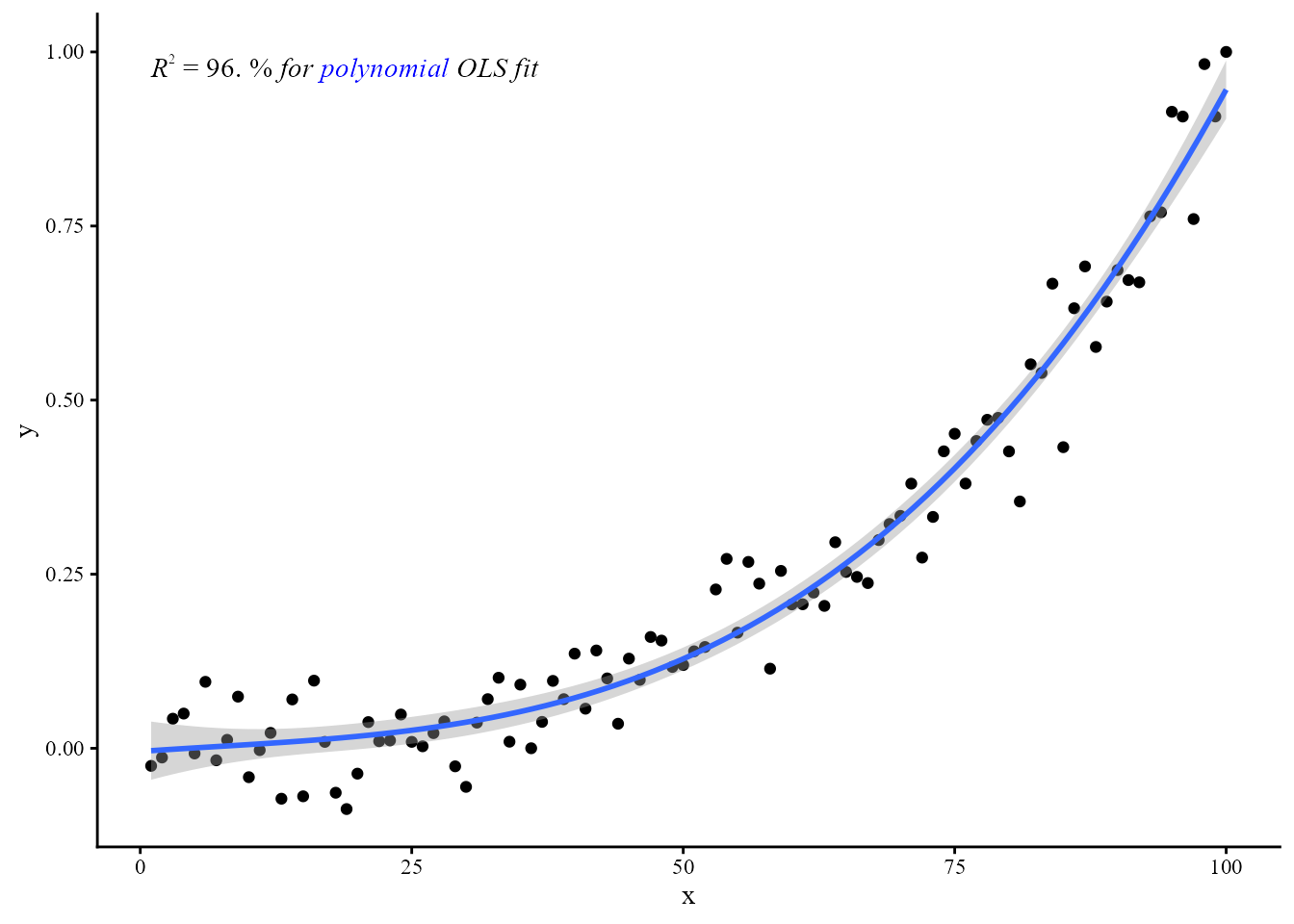
Package ‘ggpmisc’ does also export the label formatting functions used in the statistics. Using them directly can allow some additional control of the typesetting.
my.formula <- y ~ poly(x, 3, raw = TRUE)
ggplot(my.data, aes(x, y)) +
  geom_point() +
  stat_poly_line(formula = my.formula) +
  stat_poly_eq(mapping =
                 aes(label =
                       paste("$ ",
                             rr_label(value = after_stat(r.squared),
                                      pc.out = TRUE,
                                      fixed = TRUE,
                                      digits = 0,
                                      output.type = "latex"),
                             "$ \\emph{for {\\color{blue}{polynomial}} OLS fit}",
                             sep = "")),
               packages = c("xcolor", "fontspec"),
               family = "serif",
               formula = my.formula,
               geom = "latex", # needs to accept the manual markup
               output.type = "numeric",
               hjust = 0, vjust = 1)
my.formula <- y ~ poly(x, 3, raw = TRUE)
ggplot(my.data, aes(x, y)) +
  geom_point() +
  stat_poly_line(formula = my.formula) +
  stat_poly_eq(mapping =
                 aes(label =
                       paste(rr_label(value = after_stat(r.squared),
                                      pc.out = TRUE,
                                      fixed = TRUE,
                                      digits = 0,
                                      output.type = "marquee"),
                             " *for {.blue polynomial} OLS fit*", sep = "")),
               family = "serif",
               formula = my.formula,
               geom = "marquee",
               output.type = "numeric",
               hjust = 0, vjust = 1)