Non-linear model fits

Aims of ‘ggpmisc’ and caveats

Package ‘ggpmisc’ makes it easier to add to plots created using ‘ggplot2’ annotations based on fitted models and other statistics. It does this by wrapping existing model fit and other functions from base R and various R packages. The same annotations can be produced by calling the model fit functions, extracting the desired estimates and adding them to plots. There are two advantages in wrapping these functions in an extension to package ‘ggplot2’: 1) it ensures the coupling of graphical elements and the annotations by building all elements of the plot using the same data and a consistent grammar and 2) it makes it easier to annotate plots to the casual user of R, already familiar with the grammar of graphics.

To avoid confusion it is good to make clear what may seem obvious to some: if no plot is needed, then there is no reason to use this package. The values shown as annotations are not computed by ‘ggpmisc’ but instead by the usual model-fit and statistical functions from R and other packages. The same is true for model predictions, residuals, etc. that some of the functions in ‘ggpmisc’ display as lines, segments, or other graphical elements.

It is also important to remember that in most cases data analysis including exploratory and other stages should take place before annotated plots for publication are produced. Even though data analysis can benefit from combined numerical and graphical representation of the results, the use I envision for ‘ggpmisc’ is mainly for the production of plots for publication or communication. In any case, whether plots created with functions and methods from ‘ggpmisc’ are used for analysis or communication, it is crucial that users cite and refer both to ‘ggpmisc’ and to the underlying R and R packages used to fit models or to do other statistical computations.

print(citation(package = "ggpmisc", auto = TRUE), bibtex = FALSE)
#> To cite package 'ggpmisc' in publications use:
#> 
#>   Aphalo P (2026). _ggpmisc: Miscellaneous Extensions to 'ggplot2'_. R
#>   package version 0.7.0.9004,
#>   <https://docs.r4photobiology.info/ggpmisc/>.

Introduction

Layer functions in ‘ggpmisc’ can be used for fitting non-linear models, but given the diversity of possible model formulas, automatic generation of annotations for the model fit equations have not been implemented.

This article gives examples of non-linear model fits using both stat_poly_line() together with stat_poly_eq(), and with the ‘broom’ based statistics, stat_fit_augnment, stat_fit_tidy() and stat_fit_glance. In earlier version of ‘ggpmisc’ only the ‘broom’-based approach was available. However, in ‘ggpmisc’ (>= 1.0.0) stat_poly_eq() and stat_poly_line() can also be used to fit non-linear models.

Preliminaries

We load the packages used in the examples. Those imported always, and those suggested, when available.

library(ggpmisc)
#> Loading required package: ggpp
#> Loading required package: ggplot2
#> Registered S3 methods overwritten by 'ggpp':
#>   method                  from   
#>   heightDetails.titleGrob ggplot2
#>   widthDetails.titleGrob  ggplot2
#> 
#> Attaching package: 'ggpp'
#> The following object is masked from 'package:ggplot2':
#> 
#>     annotate
library(tibble)
library(dplyr)
#> 
#> Attaching package: 'dplyr'
#> The following objects are masked from 'package:stats':
#> 
#>     filter, lag
#> The following objects are masked from 'package:base':
#> 
#>     intersect, setdiff, setequal, union
library(quantreg)
#> Loading required package: SparseM

eval_onls <-  requireNamespace("onls", quietly = TRUE)
if (eval_onls) library(onls) else message("Please, install 'onls'")
#> Loading required package: minpack.lm
eval_nlme <-  requireNamespace("nlme", quietly = TRUE)
if (eval_nlme) library(nlme) else message("Please, install 'nlme'")
#> 
#> Attaching package: 'nlme'
#> The following object is masked from 'package:dplyr':
#> 
#>     collapse
eval_broom <-  requireNamespace("broom", quietly = TRUE)
if (eval_broom) library(broom) else message("Please, install 'broom'")
eval_broom_mixed <-  requireNamespace("broom.mixed", quietly = TRUE)
if (eval_broom_mixed) library(broom.mixed) else message("Please, install 'broom.mixed'")
eval_gginnards <-  requireNamespace("gginnards", quietly = TRUE)
if (eval_gginnards) library(gginnards) else message("Please, install 'gginnards'")

As we will add text and labels onto the plotting area we change the default theme to an uncluttered one with a white canvas.

old_theme <- theme_set(theme_bw())

Non linear least-squares regression

The fitting of models that are non-linear in their parameters are fit using iterative approximation algorithms, as no analytical solution is available. These methods are computation intensive, and require starting values for the estimation of parameters. Geometrically, the deviations used to compute the mean squares, are not different to those used for the analytical solution to estimation of parameters of linear models by ordinary least squares (OLS).

In R, nls() is the workhorse for non-linear least-squares regression. R also defines self starting functions describing non-linear models. These objects include both the function to be fit, and a function implementing a method of obtaining starting values for the iterative algorithm. Starting values are rough approximations, not useful by themselves, but are good enough as starting points for the search for better estimates.

Non linearity in the parameters In this context non-linearity does not refer to the shape of the fitted model when plotted. Polynomials are models linear in their parameters as these parameters are multiplier of the terms in the model equation. When the parameters being estimated appear in the model formula as power exponents, or similar, then we call such models non-linear in their parameters.

`nls()` with ‘ggpmisc’ native approach

Function SSmicmen() is a self starting function for the Michaelis-Menthen equation for the rate of a chemical reaction V as a function of the concentrtaion, C, of its precursor. It has two parameters, V_m, the asymptotic maximum V, and K, a reaction constant.

Easiest is to use formatted character strings to be parsed into plotmath expressions. We can in this case create the mapping to the label aesthetic with function use_label() (shown below) of with function f_use_label() (not shown).

micmen.formula <- y ~ SSmicmen(x, Vm, K) 
ggplot(Puromycin, aes(conc, rate, colour = state)) +
  geom_point() +
  stat_poly_line(method = "nls", 
                 formula = micmen.formula) +
  stat_poly_eq(use_label("AIC", "BIC"),
               method = "nls", 
               formula = micmen.formula,
               label.x = "centre", label.y = "bottom") +
  labs(x = "C", y = "V")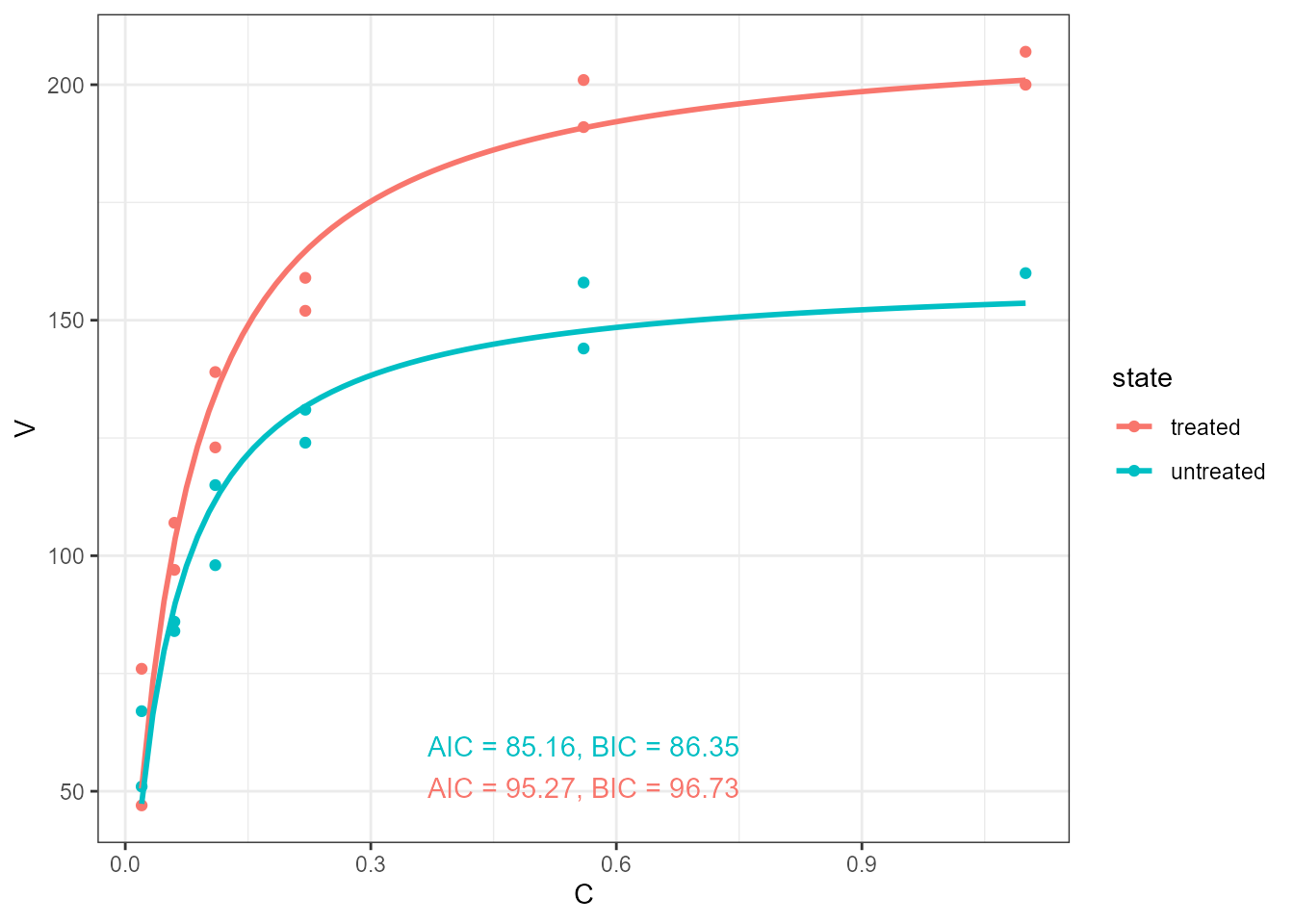

No pre-formatted equation label is available, and we have to assemble it from the numeric values of the fitted parameter estimates.

micmen.formula <- y ~ SSmicmen(x, Vm, K) 
ggplot(Puromycin, aes(conc, rate, colour = state)) +
  geom_point() +
  stat_poly_line(method = "nls", 
                 formula = micmen.formula) +
  stat_poly_eq(aes(label =
                     after_stat(
                       paste("V~`=`~frac(",
                             signif(b_0, digits = 3), "~C,",
                             signif(b_1, digits = 3), "+C)",
                             sep = ""))),
               parse = TRUE,
               method = "nls",
               output.type = "numeric",
               formula = micmen.formula,
               vstep = 0.1, size = 3,
               label.x = "centre", label.y = "bottom") +
  labs(x = "C", y = "V")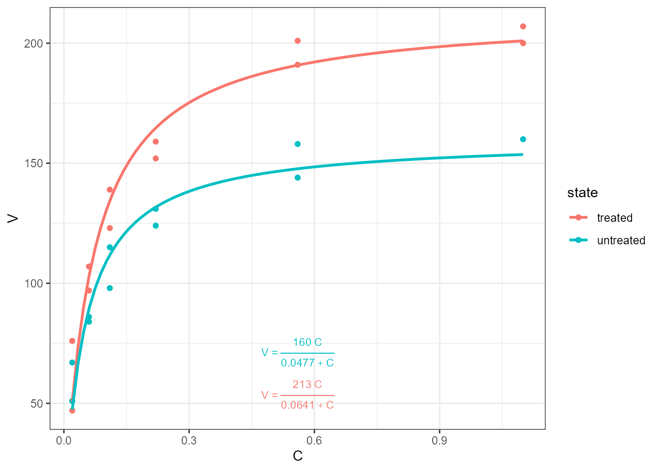

Deviations can be highlighted.

micmen.formula <- y ~ SSmicmen(x, Vm, K) 
ggplot(Puromycin, aes(conc, rate, colour = state)) +
  geom_point() +
  stat_poly_line(method = "nls", 
                 formula = micmen.formula) +
  stat_fit_deviations(
               method = "nls",
               formula = micmen.formula) +
  labs(x = "C", y = "V")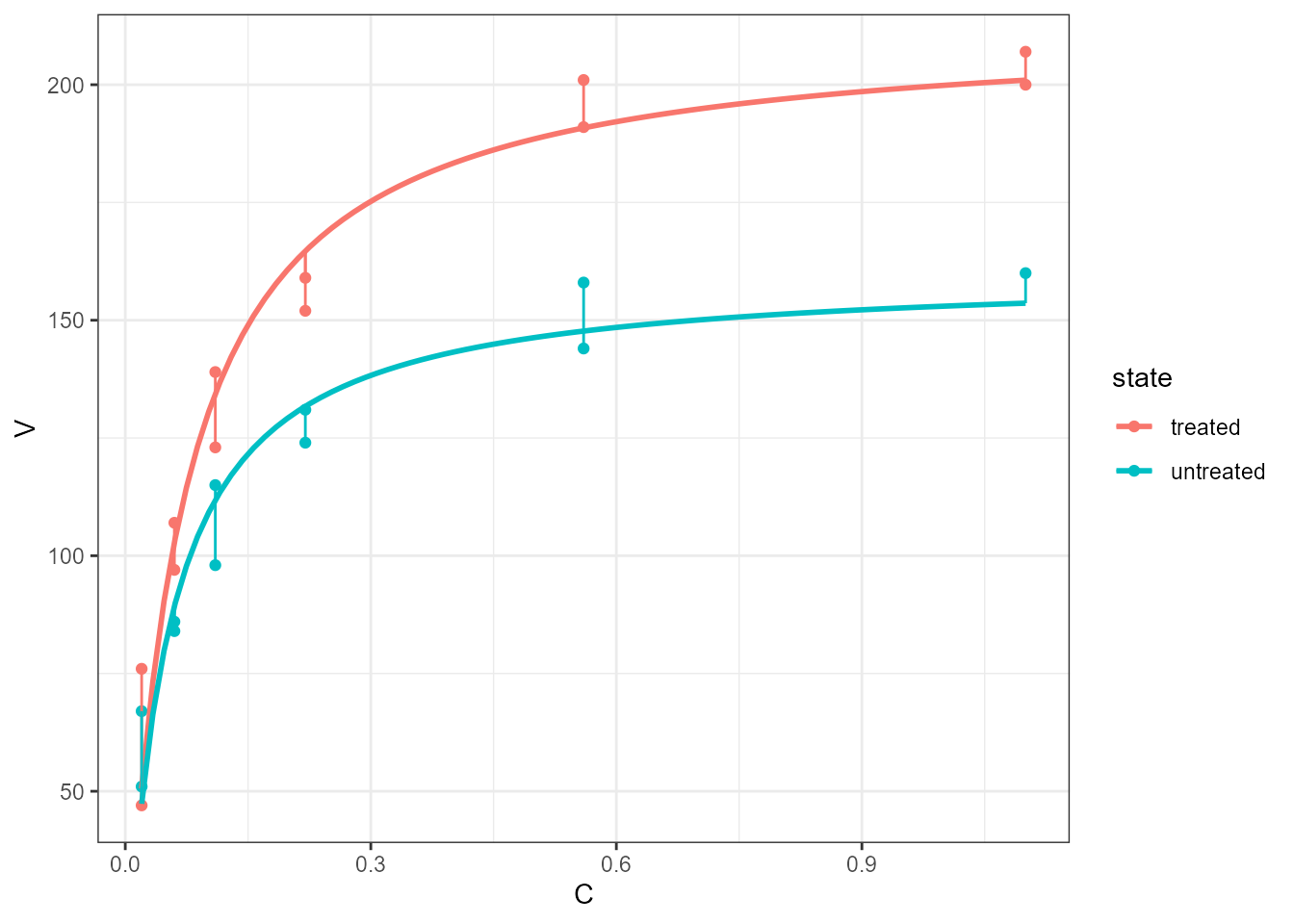

Residuals can be plotted

micmen.formula <- y ~ SSmicmen(x, Vm, K) 
ggplot(Puromycin, aes(conc, rate, colour = state)) +
  stat_fit_residuals(
               method = "nls",
               formula = micmen.formula) +
  labs(x = "C", y = "V residuals")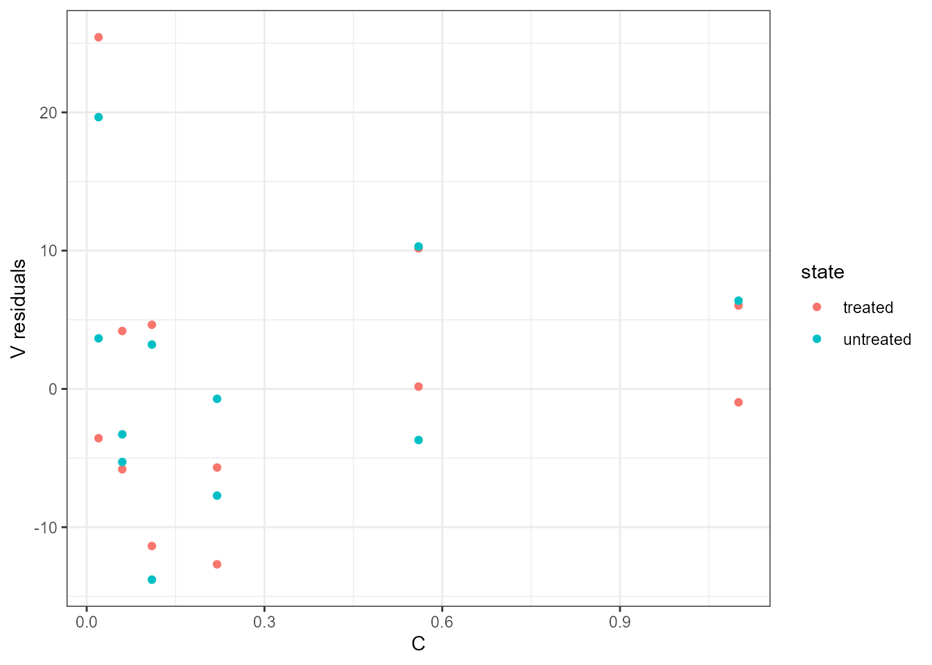

There is rarely a reason to do so, but nls() can be also used to fit linear models as it is a generally applicable procedure.

poly.formula <- y ~ b0 + b1 * x + b2 * I(x^2)
ggplot(Puromycin, aes(conc, rate, colour = state)) +
  geom_point() +
  stat_poly_line(method = "nls", 
                 method.args = list(start = list(b0 = 0, b1 = 1, b2 = 0)),
                 formula = y ~ b0 + b1 * x + b2 * I(x^2),
                 se = FALSE) +
  labs(x = "C", y = "V")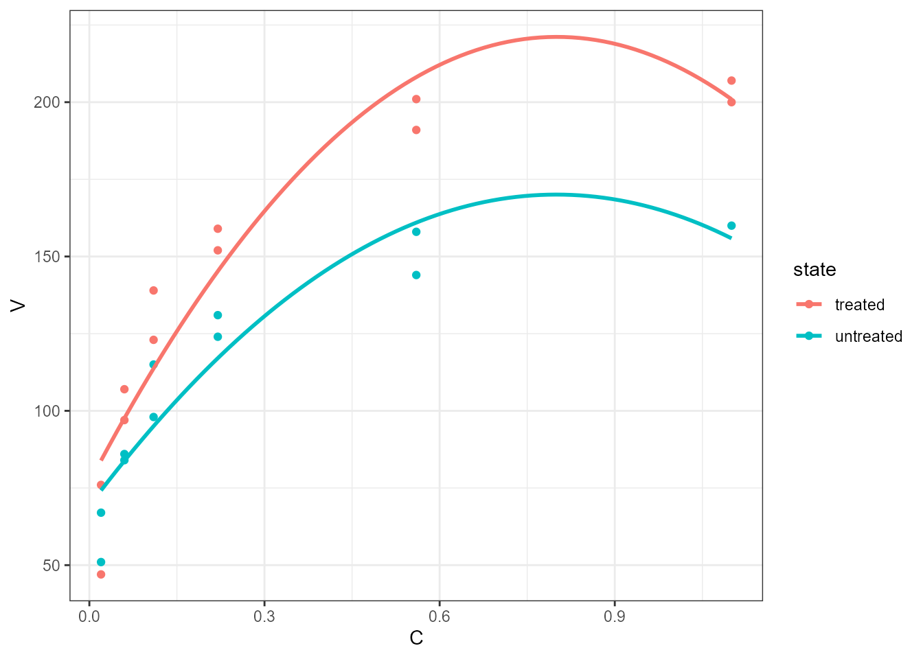

`nls()` with ‘broom’-based approach

The statistics based on methods from package ‘broom’ always return numeric values and formatted strings need to be assembled for all parameters in user’s R code within a call to aes(). The examples below produce figures nearly identical to the two first examples in the previous section.

micmen.formula <- y ~ SSmicmen(x, Vm, K) 
ggplot(Puromycin, aes(conc, rate, colour = state)) +
  geom_point() +
  stat_poly_line(method = "nls", 
                 formula = micmen.formula) +
  stat_fit_glance(aes(label = 
                        after_stat(
                          paste("AIC = ", signif(AIC, digits = 3), 
                                ", BIC = ", signif(BIC, digits = 3),
                                sep = ""))),
                  method = "nls", 
                  method.args = list(formula = micmen.formula),
                  label.x = "centre", label.y = "bottom") +
  labs(x = "C", y = "V")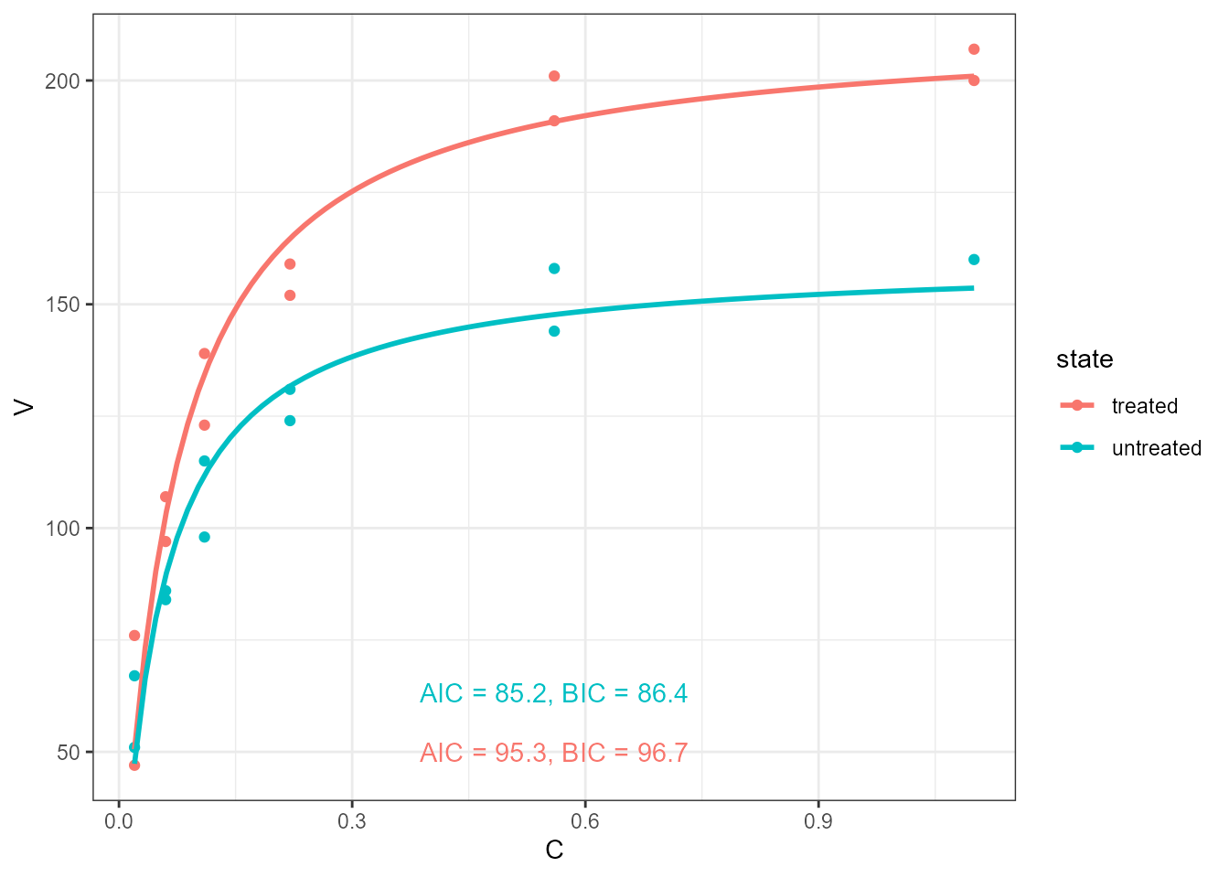

micmen.formula <- y ~ SSmicmen(x, Vm, K) 
ggplot(Puromycin, aes(conc, rate, colour = state)) +
  geom_point() +
  stat_poly_line(method = "nls", 
                 formula = micmen.formula) +
  stat_fit_tidy(aes(label =
                      after_stat(
                        paste("V~`=`~frac(",
                              signif(Vm_estimate, digits = 3), "~C,",
                              signif(K_estimate, digits = 3), "+C)",
                              sep = ""))),
                parse = TRUE,
                method = "nls", 
                method.args = list(formula = micmen.formula),
                size = 3,
                label.x = "center",
                label.y = "bottom",
                vstep = 0.12) +
  labs(x = "C", y = "V")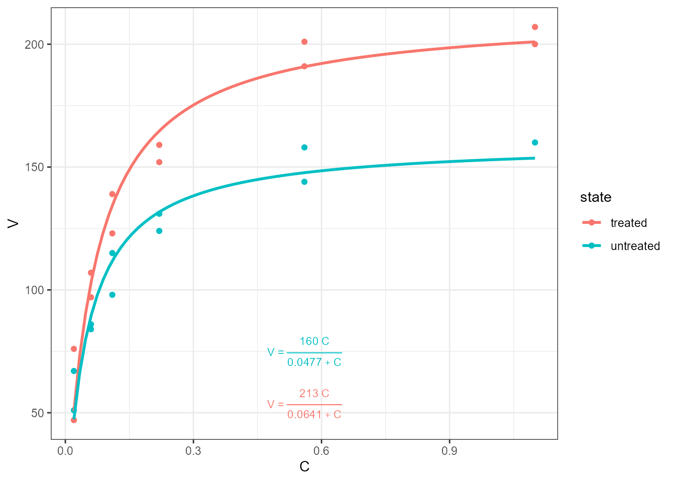

Orthogonal Nonlinear Least-Squares Regression

Orthogonal least-squares is similar in concept to model II and MA regression, but applicable to models that when plotted are curves, including models non-linear in their parameters. These methods are useful when explanatory variables are measured with error, and the intention is to describe a relationship. This is a common case in allometry (the estimation of the relative size of different parts of organs in an organism) and other data with similar properties. These and related methods, are usually described as for errors in variables (EIV) problems.

R package ‘onls’ implements function onls() that works similarly to R’s nls() but which does not make use of the self-starting estimates, which have always to be supplied explicitly.

The fit is done in two steps, NLS fit followed by the ONLS fit. The values from both fits are returned.

I use this data set here but in this context NLS is the correct approach. In fact only one of NLS or ONLS can be expected to suit a given data set. Anyway, it remains didactically useful to compare the application of both methods to the same data set.

`onls()` with ‘ggpmisc’ native approach

micmen.formula <- y ~ SSmicmen(x, Vm, K) 
ggplot(Puromycin, aes(conc, rate, colour = state)) +
  geom_point() +
  stat_poly_line(method = "onls", 
                 method.args = list(start = list(Vm = 200, K = 0.1)),
                 formula = micmen.formula) +
  stat_poly_eq(use_label("AIC", "BIC"),
               method = "onls", 
               method.args = list(start = list(Vm = 200, K = 0.1)),
               formula = micmen.formula,
               label.x = "centre", label.y = "bottom") +
  labs(x = "C", y = "V")
#> Obtaining starting parameters from ordinary NLS...
#>   Passed...
#>  Relative error in the sum of squares is at most `ftol'. 
#> Optimizing orthogonal NLS...
#>   Passed... Relative error in the sum of squares is at most `ftol'. 
#> 
#> Obtaining starting parameters from ordinary NLS...
#>   Passed...
#>  Relative error in the sum of squares is at most `ftol'. 
#> Optimizing orthogonal NLS...
#>   Passed... Relative error in the sum of squares is at most `ftol'. 
#> 
#> Obtaining starting parameters from ordinary NLS...
#>   Passed...
#>  Relative error in the sum of squares is at most `ftol'. 
#> Optimizing orthogonal NLS...
#>   Passed... Relative error in the sum of squares is at most `ftol'. 
#> 
#> Obtaining starting parameters from ordinary NLS...
#>   Passed...
#>  Relative error in the sum of squares is at most `ftol'. 
#> Optimizing orthogonal NLS...
#>   Passed... Relative error in the sum of squares is at most `ftol'.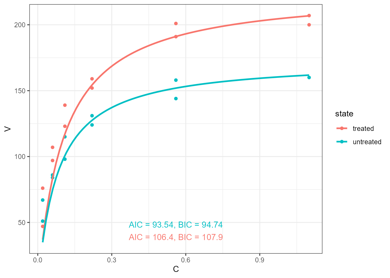

No pre-formatted equation label is available, and we have to assemble it from the numeric values of the fitted parameter estimates.

micmen.formula <- y ~ SSmicmen(x, Vm, K) 
ggplot(Puromycin, aes(conc, rate, colour = state)) +
  geom_point() +
  stat_poly_line(method = "onls", 
                 method.args = list(start = list(Vm = 200, K = 0.1)),
                 formula = micmen.formula) +
  stat_poly_eq(aes(label =
                     after_stat(
                       paste("V~`=`~frac(",
                             signif(b_0, digits = 3), "~C,",
                             signif(b_1, digits = 3), "+C)",
                             sep = ""))),
               parse = TRUE,
               method = "onls",
                 method.args = list(start = list(Vm = 200, K = 0.1)),
               output.type = "numeric",
               formula = micmen.formula,
               vstep = 0.1, size = 3,
               label.x = "centre", label.y = "bottom") +
  labs(x = "C", y = "V")
#> Obtaining starting parameters from ordinary NLS...
#>   Passed...
#>  Relative error in the sum of squares is at most `ftol'. 
#> Optimizing orthogonal NLS...
#>   Passed... Relative error in the sum of squares is at most `ftol'. 
#> 
#> Obtaining starting parameters from ordinary NLS...
#>   Passed...
#>  Relative error in the sum of squares is at most `ftol'. 
#> Optimizing orthogonal NLS...
#>   Passed... Relative error in the sum of squares is at most `ftol'. 
#> 
#> Obtaining starting parameters from ordinary NLS...
#>   Passed...
#>  Relative error in the sum of squares is at most `ftol'. 
#> Optimizing orthogonal NLS...
#>   Passed... Relative error in the sum of squares is at most `ftol'. 
#> 
#> Obtaining starting parameters from ordinary NLS...
#>   Passed...
#>  Relative error in the sum of squares is at most `ftol'. 
#> Optimizing orthogonal NLS...
#>   Passed... Relative error in the sum of squares is at most `ftol'.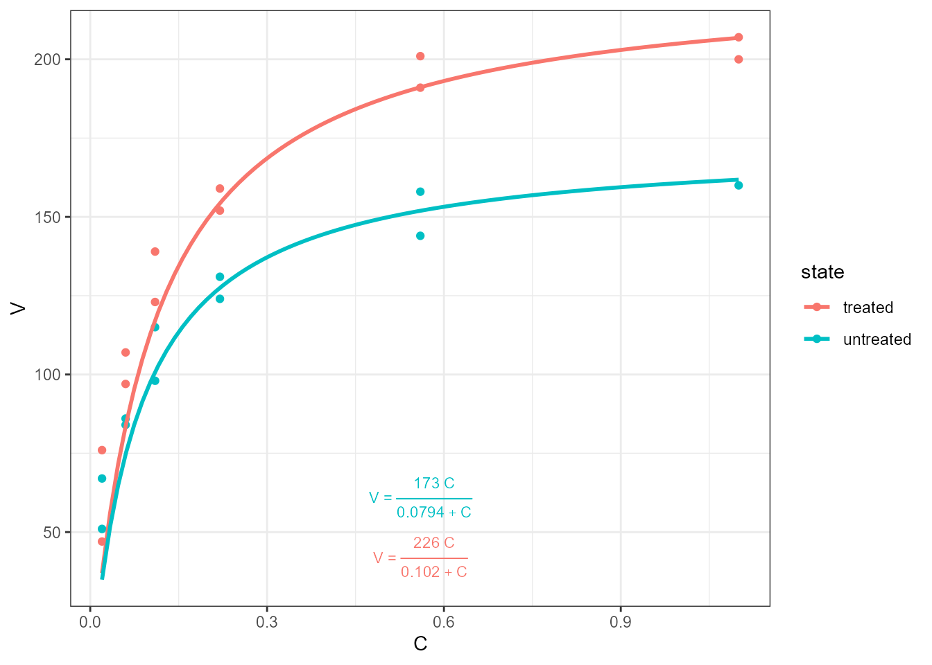

Deviations can be highlighted

So these deviations or residuals are not those whose squares have been minimized, but instead, computed as is OLS but relative to the curve fitted by ONOLS, i.e., using residuals orthogonal to the fitted curve.

micmen.formula <- y ~ SSmicmen(x, Vm, K) 
ggplot(Puromycin, aes(conc, rate, colour = state)) +
  geom_point() +
  stat_poly_line(method = "onls", 
                 method.args = list(start = list(Vm = 200, K = 0.1)),
                 formula = micmen.formula) +
  stat_fit_deviations(method = "onls",
                      method.args = list(start = list(Vm = 200, K = 0.1)),
                      formula = micmen.formula) +
  labs(x = "C", y = "V")
#> Obtaining starting parameters from ordinary NLS...
#>   Passed...
#>  Relative error in the sum of squares is at most `ftol'. 
#> Optimizing orthogonal NLS...
#>   Passed... Relative error in the sum of squares is at most `ftol'. 
#> 
#> Obtaining starting parameters from ordinary NLS...
#>   Passed...
#>  Relative error in the sum of squares is at most `ftol'. 
#> Optimizing orthogonal NLS...
#>   Passed... Relative error in the sum of squares is at most `ftol'. 
#> 
#> Obtaining starting parameters from ordinary NLS...
#>   Passed...
#>  Relative error in the sum of squares is at most `ftol'. 
#> Optimizing orthogonal NLS...
#>   Passed... Relative error in the sum of squares is at most `ftol'. 
#> 
#> Obtaining starting parameters from ordinary NLS...
#>   Passed...
#>  Relative error in the sum of squares is at most `ftol'. 
#> Optimizing orthogonal NLS...
#>   Passed... Relative error in the sum of squares is at most `ftol'.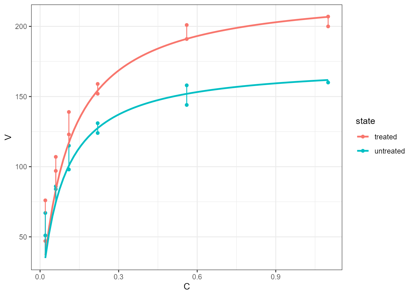

The same residuals as highlighted above can be plotted. However, these are not the orthogonal residuals used to fit the model.

micmen.formula <- y ~ SSmicmen(x, Vm, K) 
ggplot(Puromycin, aes(conc, rate, colour = state)) +
  stat_fit_residuals(
               method = "onls",
               method.args = list(start = list(Vm = 200, K = 0.1)),
               formula = micmen.formula) +
  labs(x = "C", y = "V residuals")
#> Obtaining starting parameters from ordinary NLS...
#>   Passed...
#>  Relative error in the sum of squares is at most `ftol'. 
#> Optimizing orthogonal NLS...
#>   Passed... Relative error in the sum of squares is at most `ftol'. 
#> 
#> Obtaining starting parameters from ordinary NLS...
#>   Passed...
#>  Relative error in the sum of squares is at most `ftol'. 
#> Optimizing orthogonal NLS...
#>   Passed... Relative error in the sum of squares is at most `ftol'.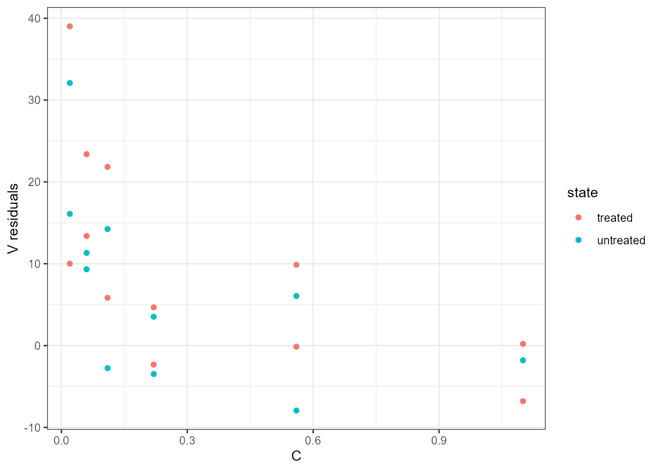

Function onls() can also be used to fit linear models using the orthogonal least-squares approach.

poly.formula <- y ~ b0 + b1 * x + b2 * I(x^2)
ggplot(Puromycin, aes(conc, rate, colour = state)) +
  geom_point() +
  stat_poly_line(method = "onls", 
                 method.args = 
                   list(start = list(b0 = 0, b1 = 1, b2 = 0)),
                 formula = poly.formula,
                 se = FALSE) +
  labs(x = "C", y = "V")
#> Obtaining starting parameters from ordinary NLS...
#>   Passed...
#>  Relative error in the sum of squares is at most `ftol'. 
#> Optimizing orthogonal NLS...
#>   Passed... Relative error in the sum of squares is at most `ftol'. 
#> 
#> Obtaining starting parameters from ordinary NLS...
#>   Passed...
#>  Relative error in the sum of squares is at most `ftol'. 
#> Optimizing orthogonal NLS...
#>   Passed... Relative error in the sum of squares is at most `ftol'.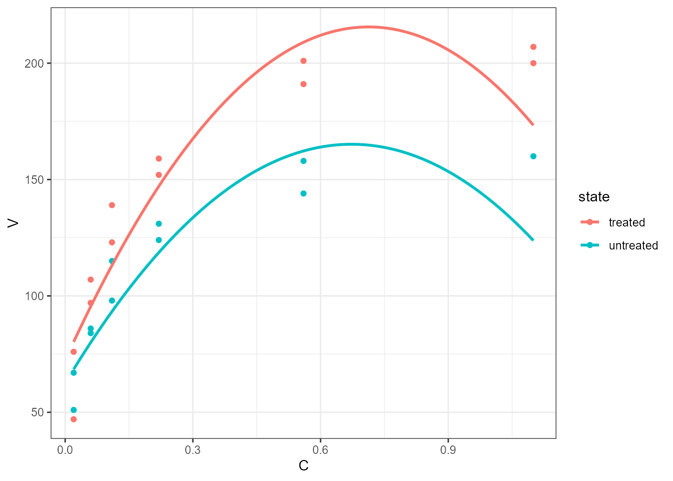

`onls()` with ‘broom’-based approach

The statistics based on methods from package ‘broom’ always return only numeric values and formatted strings need to be assembled in user’s R code within a call to aes(). The examples below produce figures nearly identical to the two first examples in the previous section.

micmen.formula <- y ~ SSmicmen(x, Vm, K) 
ggplot(Puromycin, aes(conc, rate, colour = state)) +
  geom_point() +
  stat_poly_line(method = "onls", 
                 method.args = list(start = list(Vm = 200, K = 0.1)),
                 formula = micmen.formula) +
  stat_fit_glance(aes(label = 
                        after_stat(
                          paste("AIC = ", signif(AIC, digits = 3), 
                                ", BIC = ", signif(BIC, digits = 3),
                                sep = ""))),
                  method = "onls", 
                  method.args = list(formula = micmen.formula,
                                     start = list(Vm = 200, K = 0.1)),
                  label.x = "centre", label.y = "bottom") +
  labs(x = "C", y = "V")
#> Obtaining starting parameters from ordinary NLS...
#>   Passed...
#>  Relative error in the sum of squares is at most `ftol'. 
#> Optimizing orthogonal NLS...
#>   Passed... Relative error in the sum of squares is at most `ftol'. 
#> 
#> Obtaining starting parameters from ordinary NLS...
#>   Passed...
#>  Relative error in the sum of squares is at most `ftol'. 
#> Optimizing orthogonal NLS...
#>   Passed... Relative error in the sum of squares is at most `ftol'. 
#> 
#> Obtaining starting parameters from ordinary NLS...
#>   Passed...
#>  Relative error in the sum of squares is at most `ftol'. 
#> Optimizing orthogonal NLS...
#>   Passed... Relative error in the sum of squares is at most `ftol'. 
#> 
#> Obtaining starting parameters from ordinary NLS...
#>   Passed...
#>  Relative error in the sum of squares is at most `ftol'. 
#> Optimizing orthogonal NLS...
#>   Passed... Relative error in the sum of squares is at most `ftol'.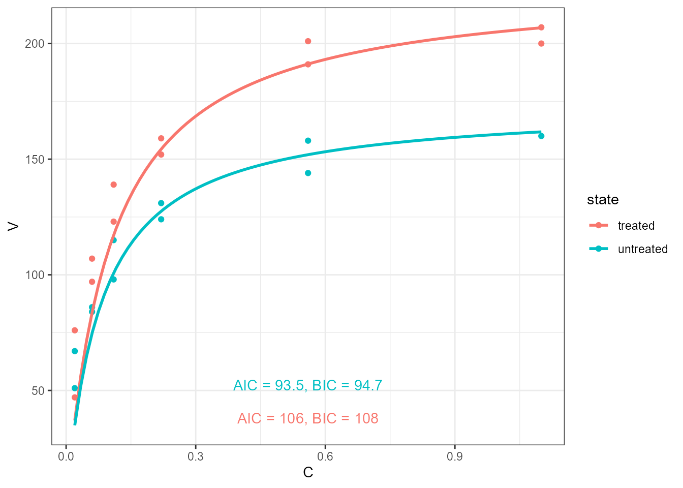

micmen.formula <- y ~ SSmicmen(x, Vm, K) 
ggplot(Puromycin, aes(conc, rate, colour = state)) +
  geom_point() +
  stat_poly_line(method = "onls", 
                 method.args = list(start = list(Vm = 200, K = 0.1)),
                 formula = micmen.formula) +
  stat_fit_tidy(aes(label =
                      after_stat(
                        paste("V~`=`~frac(",
                              signif(Vm_estimate, digits = 3), "~C,",
                              signif(K_estimate, digits = 3), "+C)",
                              sep = ""))),
                parse = TRUE,
                method = "onls", 
                method.args = list(formula = micmen.formula,
                                   start = list(Vm = 200, K = 0.1)),
                size = 3,
                label.x = "center",
                label.y = "bottom",
                vstep = 0.12) +
  labs(x = "C", y = "V")
#> Obtaining starting parameters from ordinary NLS...
#>   Passed...
#>  Relative error in the sum of squares is at most `ftol'. 
#> Optimizing orthogonal NLS...
#>   Passed... Relative error in the sum of squares is at most `ftol'. 
#> 
#> Obtaining starting parameters from ordinary NLS...
#>   Passed...
#>  Relative error in the sum of squares is at most `ftol'. 
#> Optimizing orthogonal NLS...
#>   Passed... Relative error in the sum of squares is at most `ftol'. 
#> 
#> Obtaining starting parameters from ordinary NLS...
#>   Passed...
#>  Relative error in the sum of squares is at most `ftol'. 
#> Optimizing orthogonal NLS...
#>   Passed... Relative error in the sum of squares is at most `ftol'. 
#> 
#> Obtaining starting parameters from ordinary NLS...
#>   Passed...
#>  Relative error in the sum of squares is at most `ftol'. 
#> Optimizing orthogonal NLS...
#>   Passed... Relative error in the sum of squares is at most `ftol'.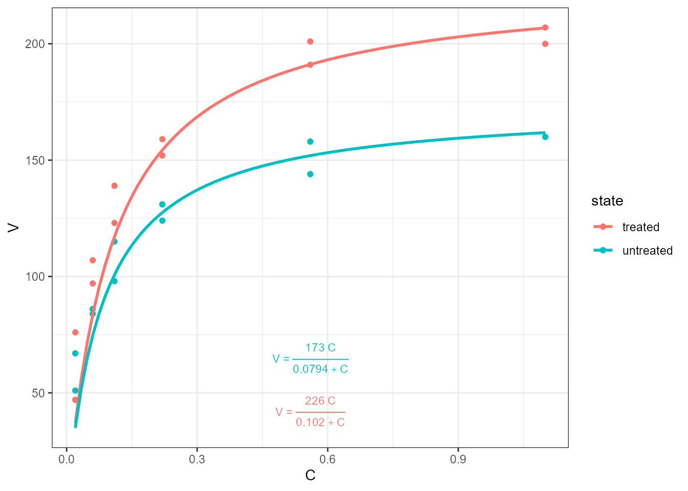

Comparison of ONLS to NLS

micmen.formula <- y ~ SSmicmen(x, Vm, K) 
ggplot(Puromycin, aes(conc, rate, colour = state)) +
  stat_poly_line(method = "nls", 
                 formula = micmen.formula,
                 linetype = "dashed",
                 limit.to = seq(0, 1.2, length.out = 80)) +
  stat_poly_line(method = "onls", 
                 method.args = list(start = list(Vm = 200, K = 0.1)),
                 formula = micmen.formula,
                 se = FALSE,
                 limit.to = seq(0, 1.2, length.out = 80)) +
  labs(x = "C", y = "V")
#> Obtaining starting parameters from ordinary NLS...
#>   Passed...
#>  Relative error in the sum of squares is at most `ftol'. 
#> Optimizing orthogonal NLS...
#>   Passed... Relative error in the sum of squares is at most `ftol'. 
#> 
#> Obtaining starting parameters from ordinary NLS...
#>   Passed...
#>  Relative error in the sum of squares is at most `ftol'. 
#> Optimizing orthogonal NLS...
#>   Passed... Relative error in the sum of squares is at most `ftol'.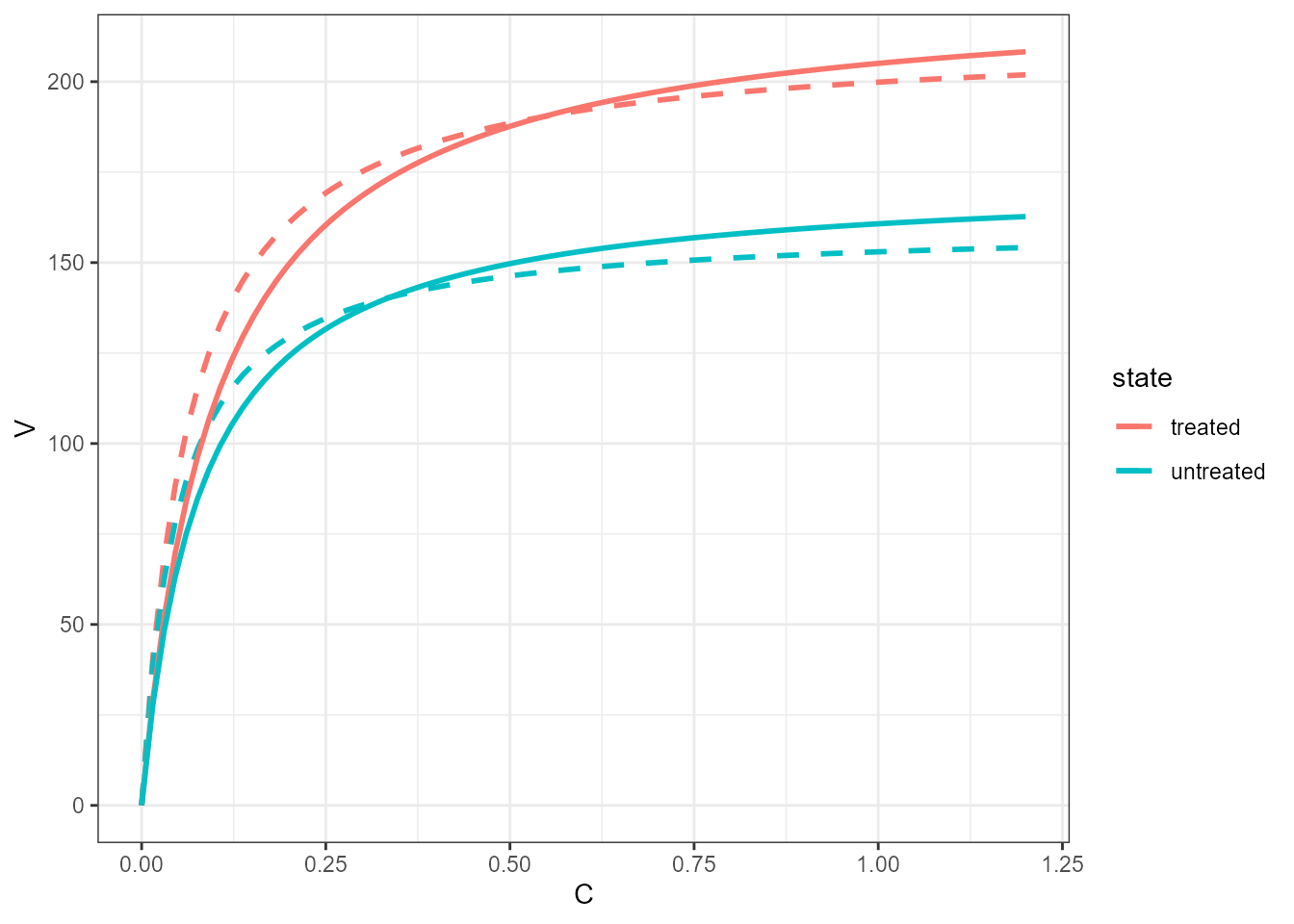

Limitations and caveats

Non-linear models are fit by approximation using an iterative approach. Convergence depends on the “goodness” of the guesses for parameter values passed as a named list to start. Solutions may be not unique and local optima can derail the search for the global best fit, and it is recommended, when not using self starting functions to repeat the fit with different starting values. When some parameter values can lead to computation errors, boundaries must be set so that the search avoids these “forbidden” conditions. In addition, different algorithms used for minimization differ in computational efficiency but also in the problems for which they may fail completly. In case of failure, it can be worthwhile to try a different algorithm.

Even if these methods are supported, model fitting can easily fail. Thus, if errors are encountered, it is necessary to run nls() or onls() on their own, to diagnose the reason of the failure to converge on a solution, arithmetic errors, or problems.

As the stats fit the model one data group at a time, when debugging, it is necessary to subset the data in the same way as ggplot() does.

fm1 <- nls(rate ~ SSmicmen(conc, Vm, K),
           data = subset(Puromycin, state == "treated"))
summary(fm1)
#> 
#> Formula: rate ~ SSmicmen(conc, Vm, K)
#> 
#> Parameters:
#>     Estimate Std. Error t value Pr(>|t|)    
#> Vm 2.127e+02  6.947e+00  30.615 3.24e-11 ***
#> K  6.412e-02  8.281e-03   7.743 1.57e-05 ***
#> ---
#> Signif. codes:  0 '***' 0.001 '**' 0.01 '*' 0.05 '.' 0.1 ' ' 1
#> 
#> Residual standard error: 10.93 on 10 degrees of freedom
#> 
#> Number of iterations to convergence: 0 
#> Achieved convergence tolerance: 1.929e-06
coef(fm1)
#>           Vm            K 
#> 212.68370727   0.06412123
predict(fm1)
#>  [1]  50.5660  50.5660 102.8110 102.8110 134.3616 134.3616 164.6847 164.6847
#>  [9] 190.8329 190.8329 200.9688 200.9688

fm2 <- onls(rate ~ SSmicmen(conc, Vm, K),
            start = list(Vm = 200, K = 0.1),
            data = subset(Puromycin, state == "treated"))
#> Obtaining starting parameters from ordinary NLS...
#>   Passed...
#>  Relative error in the sum of squares is at most `ftol'. 
#> Optimizing orthogonal NLS...
#>   Passed... Relative error in the sum of squares is at most `ftol'.
summary(fm2)
#> 
#> Formula: rate ~ SSmicmen(conc, Vm, K)
#> 
#> Parameters:
#>     Estimate Std. Error t value Pr(>|t|)    
#> Vm 226.00759   13.09763  17.256 9.04e-09 ***
#> K    0.10219    0.02046   4.995 0.000541 ***
#> ---
#> Signif. codes:  0 '***' 0.001 '**' 0.01 '*' 0.05 '.' 0.1 ' ' 1
#> 
#> Residual standard error of vertical distances: 17.41 on 10 degrees of freedom
#> Residual standard error of orthogonal distances: 0.1315 on 10 degrees of freedom
#> 
#> Number of iterations to convergence: 7 
#> Achieved convergence tolerance: 1.49e-08
coef(fm2)
#>          Vm           K 
#> 226.0075863   0.1021887
predict(fm2)
#>  [1]  36.99320  36.99320  83.60911  83.60911 117.16379 117.16379 154.32467
#>  [8] 154.32467 191.13018 191.13018 206.79644 206.79644

‘ggpmisc’ 0.7.0.9004

Pedro J. Aphalo

2026-06-16

Aims of ‘ggpmisc’ and caveats

Introduction

Preliminaries

Non linear least-squares regression

`nls()` with ‘ggpmisc’ native approach

`nls()` with ‘broom’-based approach

Orthogonal Nonlinear Least-Squares Regression

`onls()` with ‘ggpmisc’ native approach

`onls()` with ‘broom’-based approach

Comparison of ONLS to NLS

Limitations and caveats

Non-linear model fits

‘ggpmisc’ 0.7.0.9004

Pedro J. Aphalo

2026-06-16

Aims of ‘ggpmisc’ and caveats

Introduction

Preliminaries

Non linear least-squares regression

nls() with ‘ggpmisc’ native approach

nls() with ‘broom’-based approach

Orthogonal Nonlinear Least-Squares Regression

onls() with ‘ggpmisc’ native approach

onls() with ‘broom’-based approach

Comparison of ONLS to NLS

Limitations and caveats

`nls()` with ‘ggpmisc’ native approach

`nls()` with ‘broom’-based approach

`onls()` with ‘ggpmisc’ native approach

`onls()` with ‘broom’-based approach