Find the location of quantiles

Find the location of quantiles in an univariate density function, such as within a call to aes(), to map regions under the curve that the quantiles delimit to the fill aesthetic in a ggplot layer.

Usage

find_quantiles(density, quantiles = c(0.025, 0.975), group = 1)

Arguments

density

numeric A fitted density function predicted at a large number of equal steps without truncation.

quantiles

numeric The probabilities of the quantiles to locate.

group

a ‘factor’ in the sense that as.factor(f) defines the grouping, or a list of such factors in which case their interaction is used for the grouping, used in a call to split().

Value

A factor with levels indicating the regions delimited by the quantiles. The levels are labelled by ordinal numbers.

Details

A running cumulated density function (CDF) is computed as cumsum(density) assuming that x steps are uniform in size. Values are subsequently compared to the target quantiles, to identify the regions they delimit. No interpolation is done making it crucial that density is a long vector, as controlled by parameter n in stat_density().

Unique and sorted values from the argument passed to quantiles are used. Values 0 and 1 are added if not present, thus, the number of regions returned is always one less than the length of these "normalized" quantiles.

In 'ggplot2' (>= 4.0.0), geom_area() when the fill aesthetic is mapped to a numeric variable or to a factor, the fill is rendered as a gradient, making it possible to highlight multiple quantiles within a single plot layer. Gradient fills are supported in R (>= 4.1.0) and only by some graphic devices. This function is of use only if gradient fills are supported! The capabilities of the currently active device can be tested with a call to dev.capabilities() checking the field "patterns".

Function find_quantiles() is used in stat_distrmix_line() and stat_distrmix_area() to tag the regions limited by quantiles. If used on its own to create a mapping in a call to aes(), data groupings present in the ggplot must be described by the argument passed to group.

The approach used is approximate and relies on assumptions that are known to be fulfiled by the density estimates returned by specific 'ggplot2' stats such as stat_density().

Note

The approach used in find_quantiles() is very different to that used in package 'ggdensity', which is based on the local density rather than the accumulated one.

Examples

 # No grouping
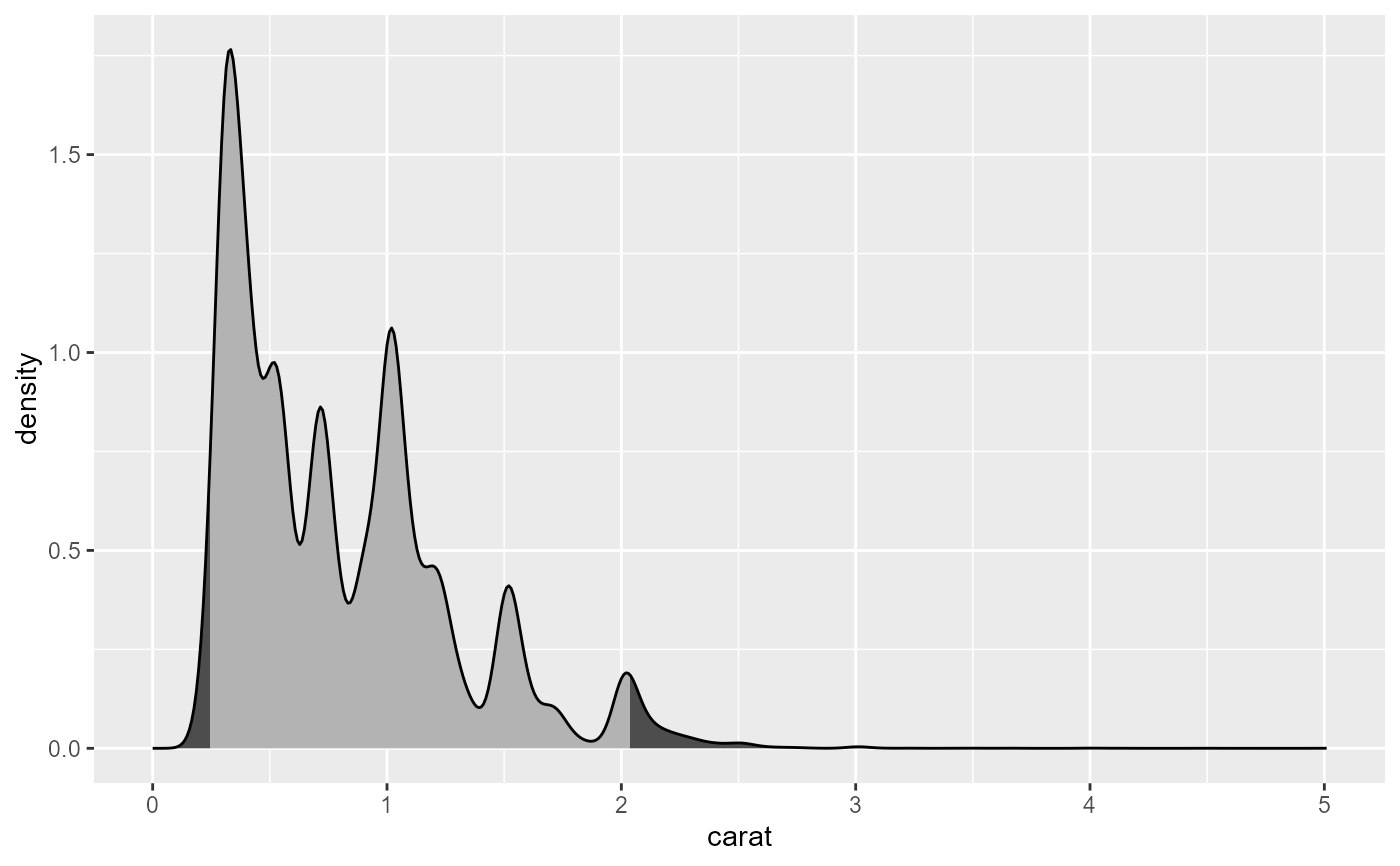
 ggplot(diamonds, aes(carat)) +
   stat_density(
     geom = "area", outline.type = "upper", colour = "black",
     aes(fill = after_stat(find_quantiles(density) != 2))) +
   scale_fill_grey(guide = "none", end = 0.3, start = 0.7) +
   expand_limits(x = 0)


 # a grouping from the mapping of cut to the fill aesthetic
 ggplot(diamonds, aes(carat, fill = cut)) +
   stat_density(
     geom = "area", outline.type = "upper", colour = "black",
     position = "stack",
     aes(alpha =
       after_stat(find_quantiles(density, c(0.1, 0.9), group) != 2)),
     show.legend = FALSE) +
   expand_limits(x = c(0, 5.5))
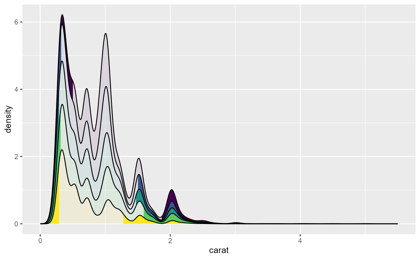
#> Warning: Using alpha for a discrete variable is not advised.